

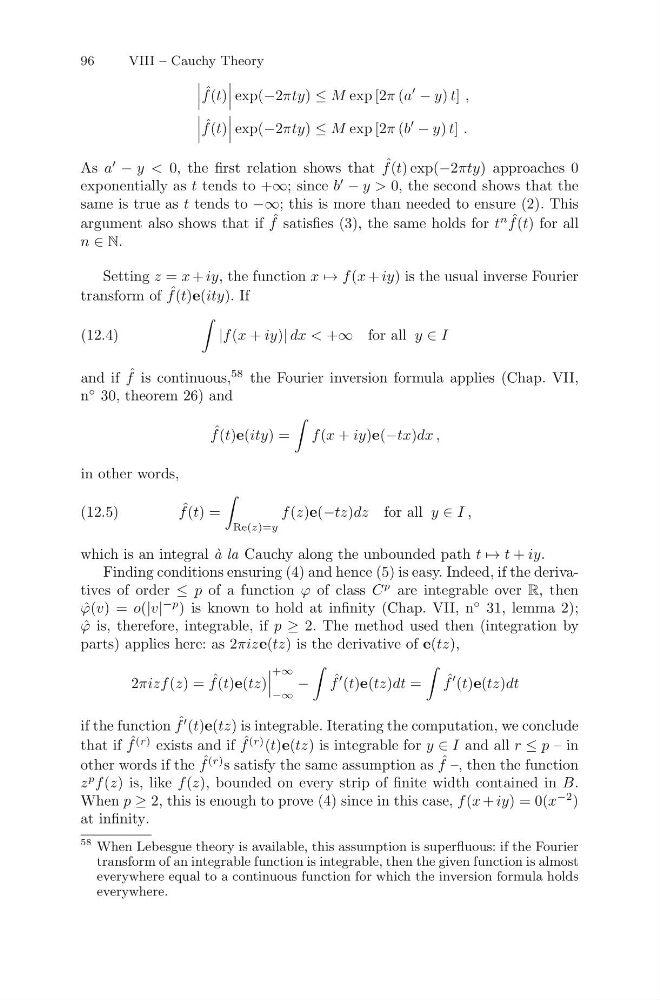
96
VIII – Cauchy Theory
ˆ
f (t)
exp(−2πty) ≤ M exp [2π (a
− y) t] ,
ˆ
f (t)
exp(−2πty) ≤ M exp [2π (b
− y) t] .
As a
− y < 0, the first relation shows that ˆ
f (t) exp(−2πty) approaches 0
exponentially as t tends to +∞; since b
− y > 0, the second shows that the
same is true as t tends to −∞; this is more than needed to ensure (2). This
argument also shows that if ˆ
f satisfies (3), the same holds for t
n ˆ
f (t) for all
n ∈ N.
Setting z = x + iy, the function x → f (x + iy) is the usual inverse Fourier
transform of ˆ
f (t)e(ity). If
|f (x + iy)| dx < +∞ for all y ∈ I
(12.4)
and if ˆ
f is continuous,
58 the Fourier inversion formula applies (Chap. VII,
n
◦ 30, theorem 26) and
ˆ
f (t)e(ity) =
f (x + iy)e(−tx)dx ,
in other words,
ˆ
f (t) =
Re(z)=y
f (z)e(−tz)dz for all y ∈ I ,
(12.5)
which is an integral ` a la Cauchy along the unbounded path t → t + iy.
Finding conditions ensuring (4) and hence (5) is easy. Indeed, if the derivatives of order ≤ p of a function ϕ of class C
p are integrable over R, then
ˆ
ϕ(v) = o(|v|
−p ) is known to hold at infinity (Chap. VII, n
◦ 31, lemma 2);
ˆ
ϕ is, therefore, integrable, if p ≥ 2. The method used then (integration by
parts) applies here: as 2πize(tz) is the derivative of e(tz),
2πizf (z) = ˆ
f (t)e(tz)
+∞
−∞
−
ˆ
f
(t)e(tz)dt =
ˆ
f
(t)e(tz)dt
if the function ˆ
f
(t)e(tz) is integrable. Iterating the computation, we conclude
that if ˆ
f
(r) exists and if ˆ
f
(r) (t)e(tz) is integrable for y ∈ I and all r ≤ p – in
other words if the ˆ
f
(r) s satisfy the same assumption as ˆ
f –, then the function
z
p f (z) is, like f (z), bounded on every strip of finite width contained in B.
When p ≥ 2, this is enough to prove (4) since in this case, f (x + iy) = 0(x
−2 )
at infinity.
58 When Lebesgue theory is available, this assumption is superfluous: if the Fourier
transform of an integrable function is integrable, then the given function is almost
everywhere equal to a continuous function for which the inversion formula holds
everywhere.
VIII – Cauchy Theory
ˆ
f (t)
exp(−2πty) ≤ M exp [2π (a
− y) t] ,
ˆ
f (t)
exp(−2πty) ≤ M exp [2π (b
− y) t] .
As a
− y < 0, the first relation shows that ˆ
f (t) exp(−2πty) approaches 0
exponentially as t tends to +∞; since b
− y > 0, the second shows that the
same is true as t tends to −∞; this is more than needed to ensure (2). This
argument also shows that if ˆ
f satisfies (3), the same holds for t
n ˆ
f (t) for all
n ∈ N.
Setting z = x + iy, the function x → f (x + iy) is the usual inverse Fourier
transform of ˆ
f (t)e(ity). If
|f (x + iy)| dx < +∞ for all y ∈ I
(12.4)
and if ˆ
f is continuous,
58 the Fourier inversion formula applies (Chap. VII,
n
◦ 30, theorem 26) and
ˆ
f (t)e(ity) =
f (x + iy)e(−tx)dx ,
in other words,
ˆ
f (t) =
Re(z)=y
f (z)e(−tz)dz for all y ∈ I ,
(12.5)
which is an integral ` a la Cauchy along the unbounded path t → t + iy.
Finding conditions ensuring (4) and hence (5) is easy. Indeed, if the derivatives of order ≤ p of a function ϕ of class C
p are integrable over R, then
ˆ
ϕ(v) = o(|v|
−p ) is known to hold at infinity (Chap. VII, n
◦ 31, lemma 2);
ˆ
ϕ is, therefore, integrable, if p ≥ 2. The method used then (integration by
parts) applies here: as 2πize(tz) is the derivative of e(tz),
2πizf (z) = ˆ
f (t)e(tz)
+∞
−∞
−
ˆ
f
(t)e(tz)dt =
ˆ
f
(t)e(tz)dt
if the function ˆ
f
(t)e(tz) is integrable. Iterating the computation, we conclude
that if ˆ
f
(r) exists and if ˆ
f
(r) (t)e(tz) is integrable for y ∈ I and all r ≤ p – in
other words if the ˆ
f
(r) s satisfy the same assumption as ˆ
f –, then the function
z
p f (z) is, like f (z), bounded on every strip of finite width contained in B.
When p ≥ 2, this is enough to prove (4) since in this case, f (x + iy) = 0(x
−2 )
at infinity.
58 When Lebesgue theory is available, this assumption is superfluous: if the Fourier
transform of an integrable function is integrable, then the given function is almost
everywhere equal to a continuous function for which the inversion formula holds
everywhere.