

Remote Sensing and Canopy Temperature
27 1
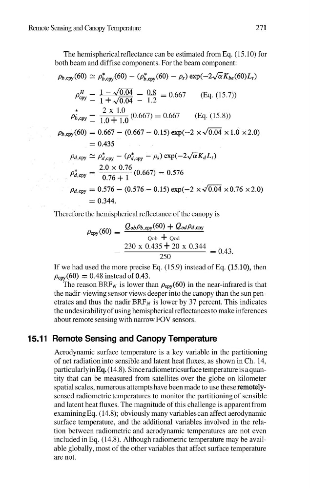
The hemispherical reflectance can be estimated from Eq. (1 5.10) for
both beam and diffise components. For the beam component:
H - 1 - r n - 0.8
- = 0.667
(Eq. (15.7))
- 1 + , m i
3 - 1.2
* - 2 x 1.0
Pb,cpy - 1 .o + 1 .o
(0.667) = 0.667
(Eq. (15.8))
Therefore the hemispherical reflectance of the canopy is
Q o b ~ b , c p y (60) + Qod~d,cpy
PCPY(6O) =
Qob + Qod
- -
230 x 0.435 + 20 x 0.344
= 0.43.
250
If we had used the more precise Eq. (15.9) instead of Eq. (15. lo), then
pcpy(60) = 0.48 instead of 0.43.
The reason BWN is lower than pcpy (60) in the near-infrared is that
the nadir-viewing sensor views deeper into the canopy than the sun penetrates and thus the nadir BRFN is lower by 37 percent. This indicates
the undesirability of using hemispherical reflectances to make inferences
about remote sensing with narrow FOV sensors.
15.1 1 Remote Sensing and Canopy Temperature
Aerodynamic surface temperature is a key variable in the partitioning
of net radiation into sensible and latent heat fluxes, as shown in Ch. 14,
particularly in Eq. (14.8). Since radiometric surface temperature is a quantity that can be measured from satellites over the globe on kilometer
spatial scales, numerous attempts have been made to use these remotelysensed radiometric temperatures to monitor the partitioning of sensible
and latent heat fluxes. The magnitude of this challenge is apparent from
examining Eq. (14.8); obviously many variables can affect aerodynamic
surface temperature, and the additional variables involved in the relation between radiometric and aerodynamic temperatures are not even
included in Eq. (14.8). Although radiometric temperature may be available globally, most of the other variables that affect surface temperature
are not.
27 1
The hemispherical reflectance can be estimated from Eq. (1 5.10) for
both beam and diffise components. For the beam component:
H - 1 - r n - 0.8
- = 0.667
(Eq. (15.7))
- 1 + , m i
3 - 1.2
* - 2 x 1.0
Pb,cpy - 1 .o + 1 .o
(0.667) = 0.667
(Eq. (15.8))
Therefore the hemispherical reflectance of the canopy is
Q o b ~ b , c p y (60) + Qod~d,cpy
PCPY(6O) =
Qob + Qod
- -
230 x 0.435 + 20 x 0.344
= 0.43.
250
If we had used the more precise Eq. (15.9) instead of Eq. (15. lo), then
pcpy(60) = 0.48 instead of 0.43.
The reason BWN is lower than pcpy (60) in the near-infrared is that
the nadir-viewing sensor views deeper into the canopy than the sun penetrates and thus the nadir BRFN is lower by 37 percent. This indicates
the undesirability of using hemispherical reflectances to make inferences
about remote sensing with narrow FOV sensors.
15.1 1 Remote Sensing and Canopy Temperature
Aerodynamic surface temperature is a key variable in the partitioning
of net radiation into sensible and latent heat fluxes, as shown in Ch. 14,
particularly in Eq. (14.8). Since radiometric surface temperature is a quantity that can be measured from satellites over the globe on kilometer
spatial scales, numerous attempts have been made to use these remotelysensed radiometric temperatures to monitor the partitioning of sensible
and latent heat fluxes. The magnitude of this challenge is apparent from
examining Eq. (14.8); obviously many variables can affect aerodynamic
surface temperature, and the additional variables involved in the relation between radiometric and aerodynamic temperatures are not even
included in Eq. (14.8). Although radiometric temperature may be available globally, most of the other variables that affect surface temperature
are not.