

Remote Sensing of Canopy Cover and IPAR
265
For our purposes, the bidirectional reflectance factor (BRF) for a
surface can be defined as follows:
flux density leaving the horizontal surface viewed by a sensor
BRF =
flux density incident on the horizontal surface
The flux density incident on the surface usually is measured by pointing the sensor at a reference surface (exposed to the same illumination
conditions as the target surface) that is as close to a perfectly-reflecting,
Lambertian surface as possible. Clearly the BRF may be different for
various wavelength bands such as the visible ( E m V ) and near-infrared
(BRFN), and the view of the sensor may be occupied by sunlit leaves,
shaded leaves, and soil (both sunlit and shaded).
If the BRF for soils and vegetation were isotropic; that is, the surfaces
responded like Lambertian surfaces, then the magnitude of the BRF would
be constant for all view angles. However the BRF for canopies can vary
by more than a factor of three with view angle for a given wavelength
band. Detailed models of canopy BRFs are complex and beyond the
scope of this book. Even analytical models such as Kuusk (1995) are
quite complicated. However, Irons et al. (1992) have represented the soil
BRF by small spheres on a flat Lambertian plane, where the shadows cast
by the spheres onto the horizontal background influence the radiation
viewed by the sensor. The BRF distributions for canopies and soils have
a characteristic shape with BRF values being highest when the sun is
directly behind the sensor and low when the sensor view is directed toward
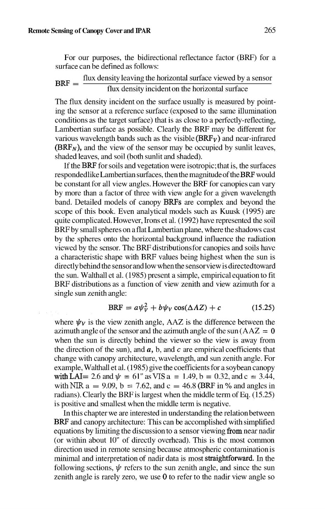
the sun. Walthall et al. (1985) present a simple, empirical equation to fit
BRF distributions as a function of view zenith and view azimuth for a
single sun zenith angle:
where +V is the view zenith angle, AAZ is the difference between the
azimuth angle of the sensor and the azimuth angle of the sun (AAZ = 0
when the sun is directly behind the viewer so the view is away from
the direction of the sun), and a, b, and c are empirical coefficients that
change with canopy architecture, wavelength, and sun zenith angle. For
example, Walthall et al. (1985) give the coefficients for a soybean canopy
withLAI= 2.6 and + = 61" as VIS a = 1.49, b = 0.32, and c = 3.44,
with NIR a = 9.09, b = 7.62, and c = 46.8 (BRF in % and angles in
radians). Clearly the BRF is largest when the middle term of Eq. (15.25)
is positive and smallest when the middle term is negative.
In this chapter we are interested in understanding the relation between
BRF and canopy architecture: This can be accomplished with simplified
equations by limiting the discussion to a sensor viewing from near nadir
(or within about 10" of directly overhead). This is the most common
direction used in remote sensing because atmospheric contamination is
minimal and interpretation of nadir data is most straightforward. In the
following sections, @ refers to the sun zenith angle, and since the sun
zenith angle is rarely zero, we use 0 to refer to the nadir view angle so
265
For our purposes, the bidirectional reflectance factor (BRF) for a
surface can be defined as follows:
flux density leaving the horizontal surface viewed by a sensor
BRF =
flux density incident on the horizontal surface
The flux density incident on the surface usually is measured by pointing the sensor at a reference surface (exposed to the same illumination
conditions as the target surface) that is as close to a perfectly-reflecting,
Lambertian surface as possible. Clearly the BRF may be different for
various wavelength bands such as the visible ( E m V ) and near-infrared
(BRFN), and the view of the sensor may be occupied by sunlit leaves,
shaded leaves, and soil (both sunlit and shaded).
If the BRF for soils and vegetation were isotropic; that is, the surfaces
responded like Lambertian surfaces, then the magnitude of the BRF would
be constant for all view angles. However the BRF for canopies can vary
by more than a factor of three with view angle for a given wavelength
band. Detailed models of canopy BRFs are complex and beyond the
scope of this book. Even analytical models such as Kuusk (1995) are
quite complicated. However, Irons et al. (1992) have represented the soil
BRF by small spheres on a flat Lambertian plane, where the shadows cast
by the spheres onto the horizontal background influence the radiation
viewed by the sensor. The BRF distributions for canopies and soils have
a characteristic shape with BRF values being highest when the sun is
directly behind the sensor and low when the sensor view is directed toward
the sun. Walthall et al. (1985) present a simple, empirical equation to fit
BRF distributions as a function of view zenith and view azimuth for a
single sun zenith angle:
where +V is the view zenith angle, AAZ is the difference between the
azimuth angle of the sensor and the azimuth angle of the sun (AAZ = 0
when the sun is directly behind the viewer so the view is away from
the direction of the sun), and a, b, and c are empirical coefficients that
change with canopy architecture, wavelength, and sun zenith angle. For
example, Walthall et al. (1985) give the coefficients for a soybean canopy
withLAI= 2.6 and + = 61" as VIS a = 1.49, b = 0.32, and c = 3.44,
with NIR a = 9.09, b = 7.62, and c = 46.8 (BRF in % and angles in
radians). Clearly the BRF is largest when the middle term of Eq. (15.25)
is positive and smallest when the middle term is negative.
In this chapter we are interested in understanding the relation between
BRF and canopy architecture: This can be accomplished with simplified
equations by limiting the discussion to a sensor viewing from near nadir
(or within about 10" of directly overhead). This is the most common
direction used in remote sensing because atmospheric contamination is
minimal and interpretation of nadir data is most straightforward. In the
following sections, @ refers to the sun zenith angle, and since the sun
zenith angle is rarely zero, we use 0 to refer to the nadir view angle so