

Water Flow in Soil
uniform, substitute from Eq. (9.3) to convert Eq. (9.20) to water potential.
Dividing through by +Lm to convert to dimensionless soil waterpotentials,
and canceling common terms, gives:
Equation (9.21) can be solved for dimensionless soil water potential and
combined with Eq. (9.19) to find a relationship between the maximum
possible uptake rate and available water in the root zone. Obtaining values
for @ ;
,
and @*,,, requires the estimation of a scaling potential @L,. If
@Lm = - 1000 J kg-', then 1.5 can be substituted for the dimensionless
permanent wilt water potential (from Fig. 9.8; +,,, = -1500 J kg-')
use 0.02 for the dimensionless field capacity, and assume b = 5 to convert
to numerical values. The resulting equation is
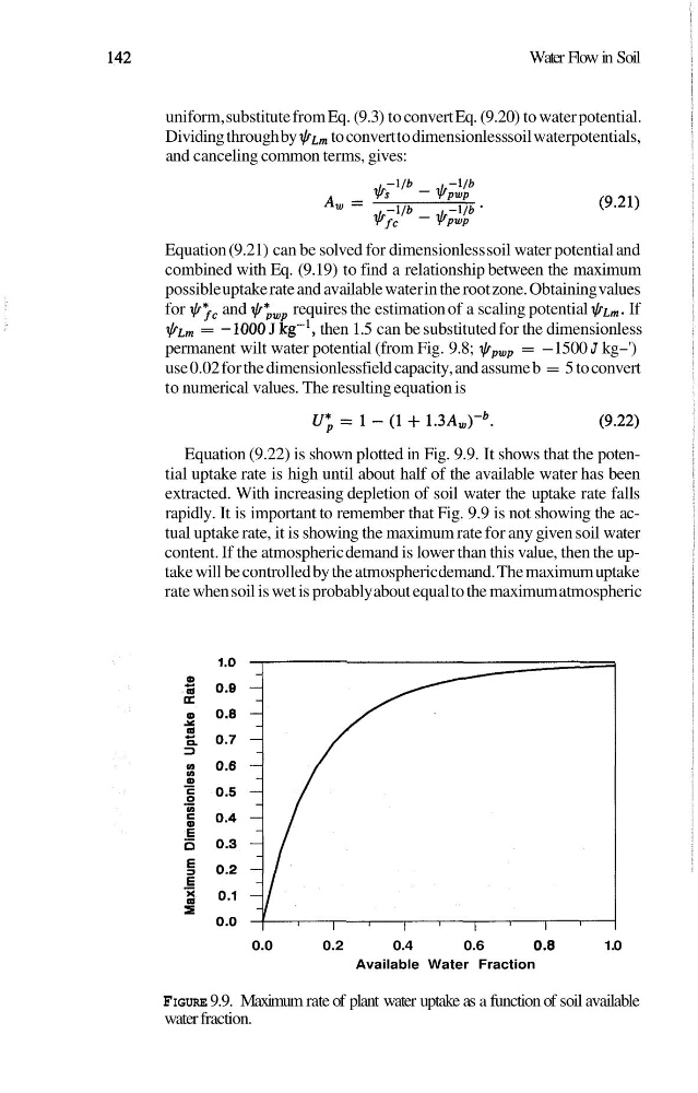
Equation (9.22) is shown plotted in Fig. 9.9. It shows that the potential uptake rate is high until about half of the available water has been
extracted. With increasing depletion of soil water the uptake rate falls
rapidly. It is important to remember that Fig. 9.9 is not showing the actual uptake rate, it is showing the maximum rate for any given soil water
content. If the atmospheric demand is lower than this value, then the uptake will be controlled by the atmospheric demand. The maximum uptake
rate when soil is wet is probably about equal to the maximum atmospheric
0.0
0.2
0.4
0.6
0.8
1.0
Available Water Fraction
FIGURE 9.9. Maximum rate of plant water uptake as a function of soil available
water fraction.
uniform, substitute from Eq. (9.3) to convert Eq. (9.20) to water potential.
Dividing through by +Lm to convert to dimensionless soil waterpotentials,
and canceling common terms, gives:
Equation (9.21) can be solved for dimensionless soil water potential and
combined with Eq. (9.19) to find a relationship between the maximum
possible uptake rate and available water in the root zone. Obtaining values
for @ ;
,
and @*,,, requires the estimation of a scaling potential @L,. If
@Lm = - 1000 J kg-', then 1.5 can be substituted for the dimensionless
permanent wilt water potential (from Fig. 9.8; +,,, = -1500 J kg-')
use 0.02 for the dimensionless field capacity, and assume b = 5 to convert
to numerical values. The resulting equation is
Equation (9.22) is shown plotted in Fig. 9.9. It shows that the potential uptake rate is high until about half of the available water has been
extracted. With increasing depletion of soil water the uptake rate falls
rapidly. It is important to remember that Fig. 9.9 is not showing the actual uptake rate, it is showing the maximum rate for any given soil water
content. If the atmospheric demand is lower than this value, then the uptake will be controlled by the atmospheric demand. The maximum uptake
rate when soil is wet is probably about equal to the maximum atmospheric
0.0
0.2
0.4
0.6
0.8
1.0
Available Water Fraction
FIGURE 9.9. Maximum rate of plant water uptake as a function of soil available
water fraction.