

76
1 From Riemann manifolds to Riemann manifolds
1-12 Equivalence theorem of equiareal mapping
The equivalence theorem of equiareal mapping from the left to the right two-dimensional Riemann
manifold (areomorphism).
We have already defined areomorphism, namely areal distortion, in order to present here an equivalence
theorem that relates areomorphism to a special partial differential equation whose solution guarantees
an equiareal mapping. In particular, we make a “canonical statement” about the product of left and
right principal stretches to be one. Furthermore, we specify the equiareal mapping for a right manifold
M
2
r , g µν
=
R
2 , δ µν
to be Euclidean.
Theorem 1.14 (Areomorphism M
2
l → M
2
r , equiareal mapping).
Let f : M
2
l → M
2
r be an orientation preserving equiareal mapping. Then the following conditions
(i)–(iv) are equivalent.
(i)
det[G l ]dU ∧ dV =
det[G r ]du ∧ dv .
(ii)
det [C r ] = det [G r ] , det [C l ] = det [G l ] , det [G r − 2E r ] = det [G r ] , det [G l + 2E l ] = det [G l ] .
(iii)
Λ 1 Λ 2 = 1 , λ 1 λ 2 = 1 .
(iv)
U u V v − U v V u =
det[G r ]
det[G l ] =
g 11 g 22 −g 2
12
G 11 G 22 −G 2
12
, u U v V − u V v U =
det[G l ]
det[G r ] =
G 11 G 22 −G 2
12
g 11 g 22 −g 2
12
.
(1.272)
End of Theorem.
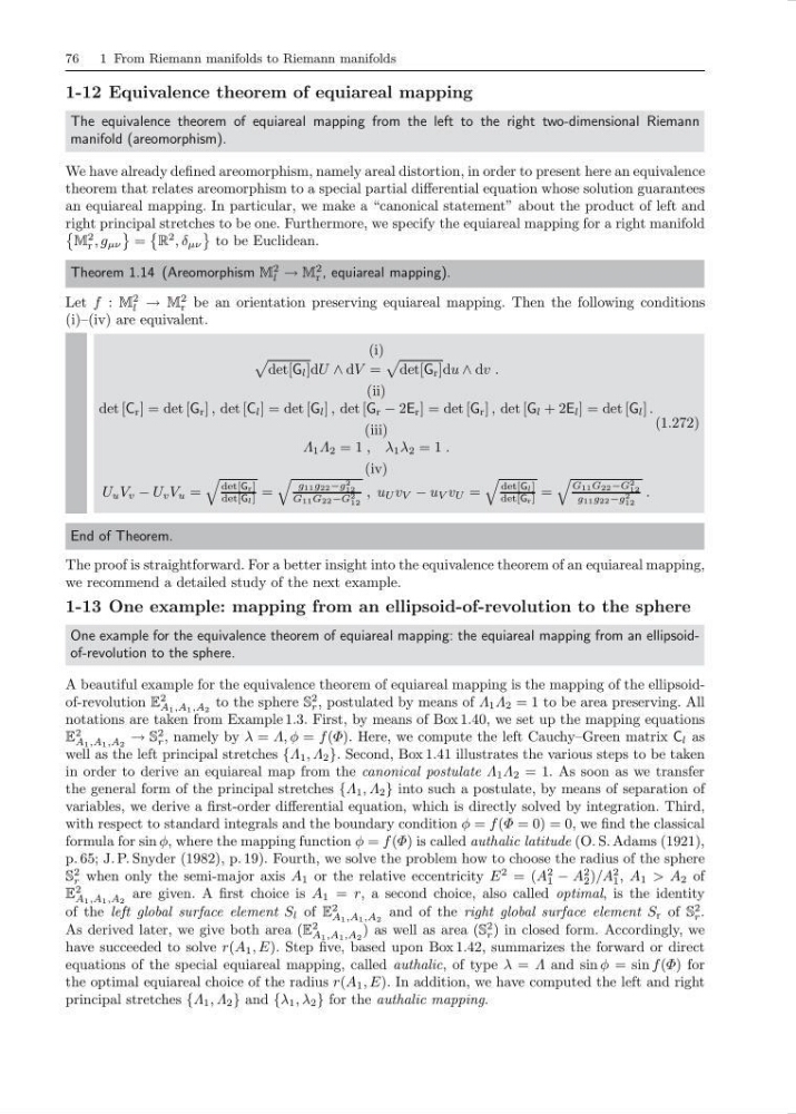
The proof is straightforward. For a better insight into the equivalence theorem of an equiareal mapping,
we recommend a detailed study of the next example.
1-13 One example: mapping from an ellipsoid-of-revolution to the sphere
One example for the equivalence theorem of equiareal mapping: the equiareal mapping from an ellipsoidof-revolution to the sphere.
A beautiful example for the equivalence theorem of equiareal mapping is the mapping of the ellipsoidof-revolution E
2
A 1 ,A 1 ,A 2
to the sphere S
2
r , postulated by means of Λ 1 Λ 2 = 1 to be area preserving. All
notations are taken from Example 1.3. First, by means of Box 1.40, we set up the mapping equations
E
2
A 1 ,A 1 ,A 2
→ S
2
r , namely by λ = Λ, φ = f (Φ). Here, we compute the left Cauchy–Green matrix C l as
well as the left principal stretches {Λ 1 , Λ 2 }. Second, Box 1.41 illustrates the various steps to be taken
in order to derive an equiareal map from the canonical postulate Λ 1 Λ 2 = 1. As soon as we transfer
the general form of the principal stretches {Λ 1 , Λ 2 } into such a postulate, by means of separation of
variables, we derive a first-order differential equation, which is directly solved by integration. Third,
with respect to standard integrals and the boundary condition φ = f (Φ = 0) = 0, we find the classical
formula for sin φ, where the mapping function φ = f (Φ) is called authalic latitude (O. S. Adams (1921),
p. 65; J. P. Snyder (1982), p. 19). Fourth, we solve the problem how to choose the radius of the sphere
S
2
r when only the semi-major axis A 1 or the relative eccentricity E
2 = (A
2
1 − A
2
2 )/A
2
1 , A 1 > A 2 of
E
2
A 1 ,A 1 ,A 2
are given. A first choice is A 1 = r, a second choice, also called optimal, is the identity
of the left global surface element S l of E
2
A 1 ,A 1 ,A 2
and of the right global surface element S r of S
2
r .
As derived later, we give both area (E
2
A 1 ,A 1 ,A 2
) as well as area (S
2
r ) in closed form. Accordingly, we
have succeeded to solve r(A 1 , E). Step five, based upon Box 1.42, summarizes the forward or direct
equations of the special equiareal mapping, called authalic, of type λ = Λ and sin φ = sin f (Φ) for
the optimal equiareal choice of the radius r(A 1 , E). In addition, we have computed the left and right
principal stretches {Λ 1 , Λ 2 } and {λ 1 , λ 2 } for the authalic mapping.
1 From Riemann manifolds to Riemann manifolds
1-12 Equivalence theorem of equiareal mapping
The equivalence theorem of equiareal mapping from the left to the right two-dimensional Riemann
manifold (areomorphism).
We have already defined areomorphism, namely areal distortion, in order to present here an equivalence
theorem that relates areomorphism to a special partial differential equation whose solution guarantees
an equiareal mapping. In particular, we make a “canonical statement” about the product of left and
right principal stretches to be one. Furthermore, we specify the equiareal mapping for a right manifold
M
2
r , g µν
=
R
2 , δ µν
to be Euclidean.
Theorem 1.14 (Areomorphism M
2
l → M
2
r , equiareal mapping).
Let f : M
2
l → M
2
r be an orientation preserving equiareal mapping. Then the following conditions
(i)–(iv) are equivalent.
(i)
det[G l ]dU ∧ dV =
det[G r ]du ∧ dv .
(ii)
det [C r ] = det [G r ] , det [C l ] = det [G l ] , det [G r − 2E r ] = det [G r ] , det [G l + 2E l ] = det [G l ] .
(iii)
Λ 1 Λ 2 = 1 , λ 1 λ 2 = 1 .
(iv)
U u V v − U v V u =
det[G r ]
det[G l ] =
g 11 g 22 −g 2
12
G 11 G 22 −G 2
12
, u U v V − u V v U =
det[G l ]
det[G r ] =
G 11 G 22 −G 2
12
g 11 g 22 −g 2
12
.
(1.272)
End of Theorem.
The proof is straightforward. For a better insight into the equivalence theorem of an equiareal mapping,
we recommend a detailed study of the next example.
1-13 One example: mapping from an ellipsoid-of-revolution to the sphere
One example for the equivalence theorem of equiareal mapping: the equiareal mapping from an ellipsoidof-revolution to the sphere.
A beautiful example for the equivalence theorem of equiareal mapping is the mapping of the ellipsoidof-revolution E
2
A 1 ,A 1 ,A 2
to the sphere S
2
r , postulated by means of Λ 1 Λ 2 = 1 to be area preserving. All
notations are taken from Example 1.3. First, by means of Box 1.40, we set up the mapping equations
E
2
A 1 ,A 1 ,A 2
→ S
2
r , namely by λ = Λ, φ = f (Φ). Here, we compute the left Cauchy–Green matrix C l as
well as the left principal stretches {Λ 1 , Λ 2 }. Second, Box 1.41 illustrates the various steps to be taken
in order to derive an equiareal map from the canonical postulate Λ 1 Λ 2 = 1. As soon as we transfer
the general form of the principal stretches {Λ 1 , Λ 2 } into such a postulate, by means of separation of
variables, we derive a first-order differential equation, which is directly solved by integration. Third,
with respect to standard integrals and the boundary condition φ = f (Φ = 0) = 0, we find the classical
formula for sin φ, where the mapping function φ = f (Φ) is called authalic latitude (O. S. Adams (1921),
p. 65; J. P. Snyder (1982), p. 19). Fourth, we solve the problem how to choose the radius of the sphere
S
2
r when only the semi-major axis A 1 or the relative eccentricity E
2 = (A
2
1 − A
2
2 )/A
2
1 , A 1 > A 2 of
E
2
A 1 ,A 1 ,A 2
are given. A first choice is A 1 = r, a second choice, also called optimal, is the identity
of the left global surface element S l of E
2
A 1 ,A 1 ,A 2
and of the right global surface element S r of S
2
r .
As derived later, we give both area (E
2
A 1 ,A 1 ,A 2
) as well as area (S
2
r ) in closed form. Accordingly, we
have succeeded to solve r(A 1 , E). Step five, based upon Box 1.42, summarizes the forward or direct
equations of the special equiareal mapping, called authalic, of type λ = Λ and sin φ = sin f (Φ) for
the optimal equiareal choice of the radius r(A 1 , E). In addition, we have computed the left and right
principal stretches {Λ 1 , Λ 2 } and {λ 1 , λ 2 } for the authalic mapping.