

1-10 Two examples: Mercator Projection and Stereographic Projection 61
In Box 1.27, we write down the metric forms “left dS
2 ” and “right ds
2 ” in the initial coordinates
{Λ, Φ} and {λ, φ}, respectively. Second, we factorize by (i) cos
2 Φ/(1 − E
2 sin
2 Φ) and (ii) cos
2 φ. The
first term A 1 dΛ and rdλ, respectively, generates dP and dp, respectively. In contrast, the second term
([A 1 (1−E
2 )/(1−E
2 sin
2 Φ)] cos Φ)dΦ and (r/ cos φ)dφ, respectively, generates dQ and dq, respectively.
Indeed, the first factors cos
2 Φ/(1 − E
2 sin
2 Φ) and cos
2 φ produce the left and the right factor of
conformality, called λ
2
l and λ
2
r , respectively. They are reciprocal to Λ
2
l and Λ
2
r , respectively. Third, by
means of Box 1.28, we aim at representing the factors of conformality, λ
2
l and λ
2
r , in terms of conformal
(isometric, isothermal) latitude Q and q, respectively, namely λ
2
l (Q) and λ
2
r (q), respectively. Here, we
have to invert the functions Q/A 1 = f (Φ) and q/r = ln tan(π/4 + φ/2) = artanh (sin φ), also called
the inverse Lambert or Gudermann function, lam or gd, respectively. φ = lam(q/r) = gd(q/r) or
sin φ = tanh(q/r), cos φ = 1/ cosh(q/r). While λ
2
l (Q) and Λ
2
l (Q) cannot be given in a closed form,
λ
2
r = 1/ cosh
2 (q/r) and Λ
2
r = cosh
2 (q/r) are available in a simple form. Fourth, by means of Box 1.29,
we prove that λ
2
r and λ
2
l , respectively, fulfill the conformal representation of the right and the left
Gaussian curvature, here written in two versions as a special Helmholtz differential equation. For
being simpler, we did first “right” followed by the more complex “left” computation. Indeed, for given
Gaussian curvature k r = 1/r
2 = constant of the sphere S
2
r and k l = (1 − E
2 sin
2 Φ)
2 /[A
2
1 (1 − E
2 )]
of the ellipsoid-of-revolution E
2
A 1 ,A 1 ,A 2
finally transformed into {q, Q} coordinates of type conformal
(isometric, isothermal), we succeed to prove ∆ ln λ
2 + 2kλ
2 = 0 of type “right” and “left”.
Solution (the fourth problem).
A “simple conformal mapping” of E
2
A 1 ,A 1 ,A 2
→ S
2
r is the isoparametric mapping characterized by
p = P , λ =
A 1
r
Λ , q = Q , A 1 ln
tan
π
4
+
Φ
2
1 − E sin Φ
1 + E sin Φ
E/2
= r ln tan
π
4
+
φ
2
. (1.222)
C. F. Gauss (1822, 1844) made some special proposals how to choose the radius r of S
2
r in an optimal
way. Here, let us refer to Chapter 2, where the Gauss projection E
2
A 1 ,A 1 ,A 2
→ S
2
r → P
2 is discussed in
detail. Here, we conclude with a representation of the left as well as the right inverse mapping Φ
−1
l
and Φ
−1
r
in terms of conformal coordinates (isometric, isothermal) of Box 1.30, which specializes Φ
−1
l
and Φ
−1
r
of Box 1.21.
End of Solution (the fourth problem).
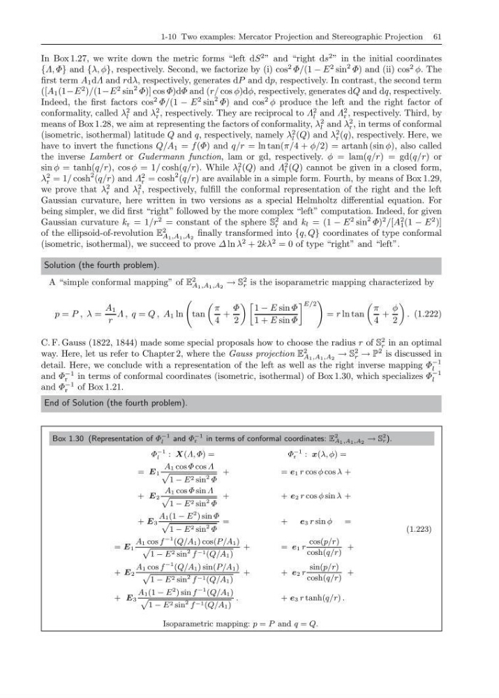
Box 1.30 (Representation of Φ
−1
l
and Φ
−1
r
in terms of conformal coordinates: E
2
A 1 ,A 1 ,A 2 → S
2
r ).
Φ
−1
l
: X (Λ, Φ) =
Φ
−1
r
: x(λ, φ) =
= E 1
A 1 cos Φ cos Λ
p
1 − E 2 sin
2 Φ
+
= e 1 r cos φ cos λ +
+ E 2
A 1 cos Φ sin Λ
p
1 − E 2 sin
2 Φ
+
+ e 2 r cos φ sin λ +
+ E 3
A 1 (1 − E
2 ) sin Φ
p
1 − E 2 sin
2 Φ
=
+
e 3 r sin φ
=
= E 1
A 1 cos f
−1 (Q/A 1 ) cos(P/A 1 )
p
1 − E 2 sin
2 f −1 (Q/A 1 )
+
= e 1 r
cos(p/r)
cosh(q/r)
+
+ E 2
A 1 cos f
−1 (Q/A 1 ) sin(P/A 1 )
p
1 − E 2 sin
2 f −1 (Q/A 1 )
+
+ e 2 r
sin(p/r)
cosh(q/r)
+
+ E 3
A 1 (1 − E
2 ) sin f
−1 (Q/A 1 )
p
1 − E 2 sin
2 f −1 (Q/A 1 )
.
+ e 3 r tanh(q/r) .
(1.223)
Isoparametric mapping: p = P and q = Q.
In Box 1.27, we write down the metric forms “left dS
2 ” and “right ds
2 ” in the initial coordinates
{Λ, Φ} and {λ, φ}, respectively. Second, we factorize by (i) cos
2 Φ/(1 − E
2 sin
2 Φ) and (ii) cos
2 φ. The
first term A 1 dΛ and rdλ, respectively, generates dP and dp, respectively. In contrast, the second term
([A 1 (1−E
2 )/(1−E
2 sin
2 Φ)] cos Φ)dΦ and (r/ cos φ)dφ, respectively, generates dQ and dq, respectively.
Indeed, the first factors cos
2 Φ/(1 − E
2 sin
2 Φ) and cos
2 φ produce the left and the right factor of
conformality, called λ
2
l and λ
2
r , respectively. They are reciprocal to Λ
2
l and Λ
2
r , respectively. Third, by
means of Box 1.28, we aim at representing the factors of conformality, λ
2
l and λ
2
r , in terms of conformal
(isometric, isothermal) latitude Q and q, respectively, namely λ
2
l (Q) and λ
2
r (q), respectively. Here, we
have to invert the functions Q/A 1 = f (Φ) and q/r = ln tan(π/4 + φ/2) = artanh (sin φ), also called
the inverse Lambert or Gudermann function, lam or gd, respectively. φ = lam(q/r) = gd(q/r) or
sin φ = tanh(q/r), cos φ = 1/ cosh(q/r). While λ
2
l (Q) and Λ
2
l (Q) cannot be given in a closed form,
λ
2
r = 1/ cosh
2 (q/r) and Λ
2
r = cosh
2 (q/r) are available in a simple form. Fourth, by means of Box 1.29,
we prove that λ
2
r and λ
2
l , respectively, fulfill the conformal representation of the right and the left
Gaussian curvature, here written in two versions as a special Helmholtz differential equation. For
being simpler, we did first “right” followed by the more complex “left” computation. Indeed, for given
Gaussian curvature k r = 1/r
2 = constant of the sphere S
2
r and k l = (1 − E
2 sin
2 Φ)
2 /[A
2
1 (1 − E
2 )]
of the ellipsoid-of-revolution E
2
A 1 ,A 1 ,A 2
finally transformed into {q, Q} coordinates of type conformal
(isometric, isothermal), we succeed to prove ∆ ln λ
2 + 2kλ
2 = 0 of type “right” and “left”.
Solution (the fourth problem).
A “simple conformal mapping” of E
2
A 1 ,A 1 ,A 2
→ S
2
r is the isoparametric mapping characterized by
p = P , λ =
A 1
r
Λ , q = Q , A 1 ln
tan
π
4
+
Φ
2
1 − E sin Φ
1 + E sin Φ
E/2
= r ln tan
π
4
+
φ
2
. (1.222)
C. F. Gauss (1822, 1844) made some special proposals how to choose the radius r of S
2
r in an optimal
way. Here, let us refer to Chapter 2, where the Gauss projection E
2
A 1 ,A 1 ,A 2
→ S
2
r → P
2 is discussed in
detail. Here, we conclude with a representation of the left as well as the right inverse mapping Φ
−1
l
and Φ
−1
r
in terms of conformal coordinates (isometric, isothermal) of Box 1.30, which specializes Φ
−1
l
and Φ
−1
r
of Box 1.21.
End of Solution (the fourth problem).
Box 1.30 (Representation of Φ
−1
l
and Φ
−1
r
in terms of conformal coordinates: E
2
A 1 ,A 1 ,A 2 → S
2
r ).
Φ
−1
l
: X (Λ, Φ) =
Φ
−1
r
: x(λ, φ) =
= E 1
A 1 cos Φ cos Λ
p
1 − E 2 sin
2 Φ
+
= e 1 r cos φ cos λ +
+ E 2
A 1 cos Φ sin Λ
p
1 − E 2 sin
2 Φ
+
+ e 2 r cos φ sin λ +
+ E 3
A 1 (1 − E
2 ) sin Φ
p
1 − E 2 sin
2 Φ
=
+
e 3 r sin φ
=
= E 1
A 1 cos f
−1 (Q/A 1 ) cos(P/A 1 )
p
1 − E 2 sin
2 f −1 (Q/A 1 )
+
= e 1 r
cos(p/r)
cosh(q/r)
+
+ E 2
A 1 cos f
−1 (Q/A 1 ) sin(P/A 1 )
p
1 − E 2 sin
2 f −1 (Q/A 1 )
+
+ e 2 r
sin(p/r)
cosh(q/r)
+
+ E 3
A 1 (1 − E
2 ) sin f
−1 (Q/A 1 )
p
1 − E 2 sin
2 f −1 (Q/A 1 )
.
+ e 3 r tanh(q/r) .
(1.223)
Isoparametric mapping: p = P and q = Q.