

I-1 The optimal Mercator projection (UM) 625
Lemma I.2 (Generalized Mercator projection, principal stretches).
With respect to the left Tissot distortion measure represented by the matrix C l G
−1
l
of the left Cauchy–
Green deformation tensor C l = J
T
l G r J l multiplied by the inverse of the left metric tensor G l , the matrix
of the metric tensor of E
2
A 1 ,A 2
, the left principal stretches of the generalized Mercator projection are
given by
Λ 1 = Λ 2 = ρ
1 − E 2 sin
2 Φ
cos Φ
.
(I.3)
The eigenvalues {Λ 1 , Λ 2 } cover the eigenspace of the left Tissot matrix C l G
−1
l . Due to conformality,
they are identical, Λ 1 = Λ 2 = Λ S . J l denotes the left Jacobi map (dx, dy) → (dΛ, dΦ), G r the matrix
of the right metric tensor of the plane generated by developing the circular cylinder C
2
ρA 1
of radius
ρA 1 , namely the unit matrix G r = I 2 .
End of Lemma.
Definition I.3 (Generalized Mercator projection, Airy optimum).
The generalized Mercator projection of the ellipsoid-of-revolution E
2
A 1 ,A 2
onto the developed circular
cylinder C
2
ρA 1
of radius ρA 1 is called Airy optimal if the deviation from an isometry (I.4) in terms
of the left principal stretches {Λ 1 , Λ 2 } averaged over a mapping area of interest, namely the surface
integral (I.5), is minimal with respect to the unknown dilatation factor ρ.
(Λ 1 − 1)
2 + (Λ 2 − 1)
2
2
,
(I.4)
J lA :=
1
2S
area
(Λ 1 − 1)
2 + (Λ 2 − 1)
2
dS = min
ρ
.
(I.5)
End of Definition.
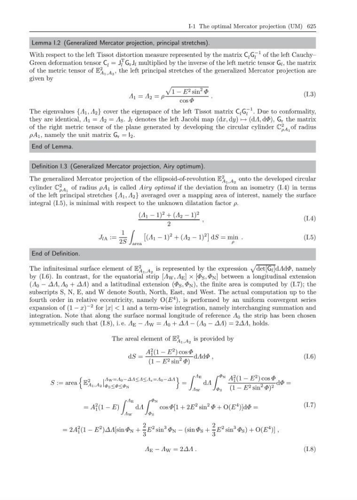
The infinitesimal surface element of E
2
A 1 ,A 2
is represented by the expression
det[G l ]dΛdΦ, namely
by (I.6). In contrast, for the equatorial strip [Λ W , Λ E ] × [Φ S , Φ N ] between a longitudinal extension
(Λ 0 − ∆Λ, Λ 0 + ∆Λ) and a latitudinal extension (Φ S , Φ N ), the finite area is computed by (I.7); the
subscripts S, N, E, and W denote South, North, East, and West. The actual computation up to the
fourth order in relative eccentricity, namely O(E
4 ), is performed by an uniform convergent series
expansion of (1 − x)
−2 for |x| < 1 and a term-wise integration, namely interchanging summation and
integration. Note that along the surface normal longitude of reference Λ 0 the strip has been chosen
symmetrically such that (I.8), i. e. Λ E − Λ W = Λ 0 + ∆Λ − (Λ 0 − ∆Λ) = 2∆Λ, holds.
The areal element of E
2
A 1 ,A 2
is provided by
dS =
A
2
1 (1 − E
2 ) cos Φ
(1 − E 2 sin
2 Φ)
dΛdΦ ,
(I.6)
S := area
E
2
A 1 ,A 2
Λ W =Λ 0 −∆Λ≤Λ≤Λ ε =Λ 0 −∆Λ
Φ S ≤Φ≤Φ N
=
Λ E
Λ W
dΛ
Φ N
Φ S
A
2
1 (1 − E
2 ) cos Φ
(1 − E 2 sin
2 Φ) 2 dΦ =
= A
2
1 (1 − E)
Λ E
Λ W
dΛ
Φ N
Φ S
cos Φ[1 + 2E
2 sin
2 Φ + O(E
4 )]dΦ =
= 2A
2
1 (1 − E
2 )∆Λ[sin Φ N +
2
3
E
2 sin
3 Φ N − (sin Φ S +
2
3
E
2 sin
3 Φ S ) + O(E
4 )] ,
(I.7)
Λ E − Λ W = 2∆Λ .
(I.8)