

H-2 The ellipsoidal Hammer projection 613
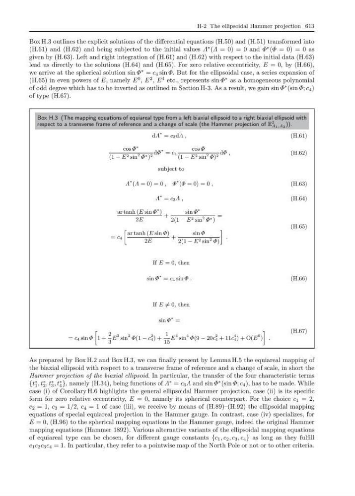
Box H.3 outlines the explicit solutions of the differential equations (H.50) and (H.51) transformed into
(H.61) and (H.62) and being subjected to the initial values Λ
∗ (Λ = 0) = 0 and Φ
∗ (Φ = 0) = 0 as
given by (H.63). Left and right integration of (H.61) and (H.62) with respect to the initial data (H.63)
lead us directly to the solutions (H.64) and (H.65). For zero relative eccentricity, E = 0, by (H.66),
we arrive at the spherical solution sin Φ
∗ = c 4 sin Φ. But for the ellipsoidal case, a series expansion of
(H.65) in even powers of E, namely E
0 , E
2 , E
4 etc., represents sin Φ
∗ as a homogeneous polynomial
of odd degree which has to be inverted as outlined in Section H-3. As a result, we gain sin Φ
∗ (sin Φ; c 4 )
of type (H.67).
Box H.3 (The mapping equations of equiareal type from a left biaxial ellipsoid to a right biaxial ellipsoid with
respect to a transverse frame of reference and a change of scale (the Hammer projection of E
2
A 1 ,A 2 )).
dΛ
∗ = c 3 dΛ ,
(H.61)
cos Φ
∗
(1 − E 2 sin
2 Φ ∗ ) 2 dΦ
∗ = c 4
cos Φ
(1 − E 2 sin
2 Φ) 2 dΦ ,
(H.62)
subject to
Λ
∗ (Λ = 0) = 0 , Φ
∗ (Φ = 0) = 0 ,
(H.63)
Λ
∗ = c 3 Λ ,
(H.64)
ar tanh (E sin Φ
∗ )
2E
+
sin Φ
∗
2(1 − E 2 sin
2 Φ ∗ )
=
= c 4
»
ar tanh (E sin Φ)
2E
+
sin Φ
2(1 − E 2 sin
2 Φ)
–
.
(H.65)
If E = 0, then
sin Φ
∗ = c 4 sin Φ .
(H.66)
If E = 0, then
sin Φ
∗ =
= c 4 sin Φ
»
1 +
2
3
E
2 sin
2 Φ(1 − c
2
4 ) +
1
15
E
4 sin
4 Φ(9 − 20c
2
4 + 11c
4
4 ) + O(E
6 )
–
.
(H.67)
As prepared by Box H.2 and Box H.3, we can finally present by Lemma H.5 the equiareal mapping of
the biaxial ellipsoid with respect to a transverse frame of reference and a change of scale, in short the
Hammer projection of the biaxial ellipsoid. In particular, the transfer of the four characteristic terms
{t
∗
1 , t
∗
2 , t
∗
3 , t
∗
4 }, namely (H.34), being functions of Λ
∗ = c 3 Λ and sin Φ
∗ (sin Φ; c 4 ), has to be made. While
case (i) of Corollary H.6 highlights the general ellipsoidal Hammer projection, case (ii) is its specific
form for zero relative eccentricity, E = 0, namely its spherical counterpart. For the choice c 1 = 2,
c 2 = 1, c 3 = 1/2, c 4 = 1 of case (iii), we receive by means of (H.89)–(H.92) the ellipsoidal mapping
equations of special equiareal projection in the Hammer gauge. In contrast, case (iv) specializes, for
E = 0, (H.96) to the spherical mapping equations in the Hammer gauge, indeed the original Hammer
mapping equations (Hammer 1892). Various alternative variants of the ellipsoidal mapping equations
of equiareal type can be chosen, for different gauge constants {c 1 , c 2 , c 3 , c 4 } as long as they fulfill
c 1 c 2 c 3 c 4 = 1. In particular, they refer to a pointwise map of the North Pole or not or to other criteria.