

42
1 From Riemann manifolds to Riemann manifolds
Box 1.23 (Relative angular shear).
Left Cauchy–Green matrix:
Right Cauchy–Green matrix:
C l =
»
r
2 cos
2 Φ 0
0
r
2
–
.
C r =
2
6
6
6
4
A 1 cos
2 φ
1 − E 2 sin
2 φ
0
0
A
2
1
`
1 − E
2
´ 2
`
1 − E 2 sin
2 φ
´ 3
3
7
7
7
5
.
(1.150)
Left angular shear:
Right angular shear:
cos Ψ l =
˙
u
T
1 C r ˙
u 2
˙
u 1 C r ˙
u 2 C r
,
cos Ψ r =
˙
U
T
1 C l ˙
U 2
˙
U 1 C l ˙
U 2 C l
,
cos Ψ l ∼ [1, 0] C r
»
0
1
–
= 0 ,
cos Ψ r ∼ [1, 0] C l
»
0
1
–
= 0 ,
cos Ψ l = 0 ⇔ Ψ l = ±
π
2
.
cos Ψ r = 0 ⇔ Ψ r = ±
π
2
.
(1.151)
Left relative angular shear:
Right relative angular shear:
Q l :=
cos Ψ r
cos Ψ l
= 1 .
Q r :=
cos Ψ l
cos Ψ r
= 1 .
(1.152)
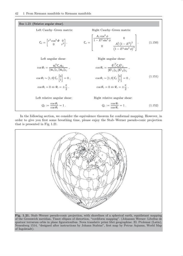
In the following section, we consider the equivalence theorem for conformal mapping. However, in
order to give you first some breathing time, please enjoy the Stab–Werner pseudo-conic projection
that is presented in Fig. 1.21.
Fig. 1.21. Stab–Werner pseudo-conic projection, with shorelines of a spherical earth, equidistant mapping
of the Greenwich meridian, Tissot ellipses of distortion, “cordiform mapping”. (Johannes Werner: Libellus de
quatuor terrarum orbis in plane figurationibus. Nova translativ primi libri geographiae. El. Ptolemai (Latin),
Nenenberg 1514, “designed after instructions by Johann Stabius”, first map by Petrus Aqianus, World Map
of Ingolstadt).
1 From Riemann manifolds to Riemann manifolds
Box 1.23 (Relative angular shear).
Left Cauchy–Green matrix:
Right Cauchy–Green matrix:
C l =
»
r
2 cos
2 Φ 0
0
r
2
–
.
C r =
2
6
6
6
4
A 1 cos
2 φ
1 − E 2 sin
2 φ
0
0
A
2
1
`
1 − E
2
´ 2
`
1 − E 2 sin
2 φ
´ 3
3
7
7
7
5
.
(1.150)
Left angular shear:
Right angular shear:
cos Ψ l =
˙
u
T
1 C r ˙
u 2
˙
u 1 C r ˙
u 2 C r
,
cos Ψ r =
˙
U
T
1 C l ˙
U 2
˙
U 1 C l ˙
U 2 C l
,
cos Ψ l ∼ [1, 0] C r
»
0
1
–
= 0 ,
cos Ψ r ∼ [1, 0] C l
»
0
1
–
= 0 ,
cos Ψ l = 0 ⇔ Ψ l = ±
π
2
.
cos Ψ r = 0 ⇔ Ψ r = ±
π
2
.
(1.151)
Left relative angular shear:
Right relative angular shear:
Q l :=
cos Ψ r
cos Ψ l
= 1 .
Q r :=
cos Ψ l
cos Ψ r
= 1 .
(1.152)
In the following section, we consider the equivalence theorem for conformal mapping. However, in
order to give you first some breathing time, please enjoy the Stab–Werner pseudo-conic projection
that is presented in Fig. 1.21.
Fig. 1.21. Stab–Werner pseudo-conic projection, with shorelines of a spherical earth, equidistant mapping
of the Greenwich meridian, Tissot ellipses of distortion, “cordiform mapping”. (Johannes Werner: Libellus de
quatuor terrarum orbis in plane figurationibus. Nova translativ primi libri geographiae. El. Ptolemai (Latin),
Nenenberg 1514, “designed after instructions by Johann Stabius”, first map by Petrus Aqianus, World Map
of Ingolstadt).