

B-2 Inversion of a bivariate homogeneous polynomial of degree n 511
Continuation of Box.
Backward substitution:
A
B = I
⇔
2
6
6
6
6
6
6
6
4
B 11 B 12 . . . B 1n−1
B 1n
0 B 22 . . . B 2n−1
B 2n
.
. . . .
.
.
0
0 . . . B n−1n−1 B n−1n
0
0 . . .
0
B nn
3
7
7
7
7
7
7
7
5
2
6
6
6
6
6
6
6
4
A 11 A 12 . . . A 1n−1
A 1n
0 A 22 . . . A 2n−1
A 2n
.
. ...
.
.
0
0 . . . A n−1n−1 A n−1n
0
0 . . .
0
A nn
3
7
7
7
7
7
7
7
5
= I .
(B.28)
(i) B 11 A 11 = I 2 ⇒ B 11 = A
−1
11 ;
(ii) B 12 A 12 + B 12 A 22 = 0 ⇒ B 12 = −B 11 A 12 A
−1
22 = −A
−1
11 A 12 A
−1[2]
22
;
(iii) B 11 A 13 + B 12 A 23 + B 13 A 33 = 0 ⇒ B 13 = − (B 11 A 13 + B 12 A 23 ) A
−1
33 =
= A
−1
11
`
A 12 A
−1
22 A 23 − A 13
´
A
−1
33 ;
(iv) B 11 A 14 + B 12 A 24 + B 13 A 34 + B 14 A 44 = 0 ⇒ B 14 = − (B 11 A 14 + B 12 A 24 + B 13 A 34 ) A
−1
44 =
= A
−1
11
ˆ
A 12 A
−1
22
`
A 24 − A 23 A
−1
33 A 34
´
+ A 13 A
−1
33 A 34 − A 14
˜
A
−1
44 .
(B.29)
(Consult Box B.5 for the general representation of B 1n .)
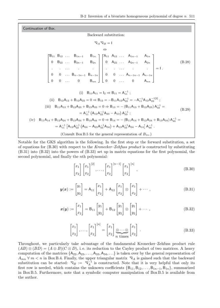
Notable for the GKS algorithm is the following. In the first step or the forward substitution, a set
of equations for (B.30) with respect to the Kronecker–Zehfuss product is constructed by substituting
(B.31) into (B.32) into the powers of (B.33) set up in matrix equations for the first polynomial, the
second polynomial, and finally the nth polynomial:
x 1
x 2
x 1
x 2
[2]
, . . . ,
x 1
x 2
[n−1]
x 1
x 2
[n]
,
(B.30)
y(x) :=
y 1
y 2
= A 11
x 1
x 2
+ A 12
x 1
x 2
⊗
x 1
x 2
+ · · · ,
(B.31)
x(y) :=
x 1
x 2
= B 11
y 1
y 2
+ B 12
y 1
y 2
⊗
y 1
y 2
+ · · · ,
(B.32)
x 1
x 2
, . . . ,
x 1
x 2
[n]
=
x 1
x 2
⊗ · · · ⊗
n times
x 1
x 2
.
(B.33)
Throughout, we particularly take advantage of the fundamental Kronecker–Zehfuss product rule
(AB) ⊗ (BD) = (A ⊗ B)(C ⊗ D), i. e. its reduction to the Cayley product of two matrices. A heavy
computation of the matrices {A 22 , A 23 , . . . , A 33 , A 34 , . . .} is taken over by the general representation of
A mn ∀ m < n in Box B.4. Finally, the upper triangular matrix A is gained such that the backward
substitution can be started: B :=
−1
A is constructed. Note that it is very helpful that only its
first row is needed, which contains the unknown coefficients {B 11 , B 12 , . . . , B 1n−1 , B 1n }, summarized
in Box B.5. Furthermore, note that a symbolic computer manipulation of Box B.5 is available from
the author.
Continuation of Box.
Backward substitution:
A
B = I
⇔
2
6
6
6
6
6
6
6
4
B 11 B 12 . . . B 1n−1
B 1n
0 B 22 . . . B 2n−1
B 2n
.
. . . .
.
.
0
0 . . . B n−1n−1 B n−1n
0
0 . . .
0
B nn
3
7
7
7
7
7
7
7
5
2
6
6
6
6
6
6
6
4
A 11 A 12 . . . A 1n−1
A 1n
0 A 22 . . . A 2n−1
A 2n
.
. ...
.
.
0
0 . . . A n−1n−1 A n−1n
0
0 . . .
0
A nn
3
7
7
7
7
7
7
7
5
= I .
(B.28)
(i) B 11 A 11 = I 2 ⇒ B 11 = A
−1
11 ;
(ii) B 12 A 12 + B 12 A 22 = 0 ⇒ B 12 = −B 11 A 12 A
−1
22 = −A
−1
11 A 12 A
−1[2]
22
;
(iii) B 11 A 13 + B 12 A 23 + B 13 A 33 = 0 ⇒ B 13 = − (B 11 A 13 + B 12 A 23 ) A
−1
33 =
= A
−1
11
`
A 12 A
−1
22 A 23 − A 13
´
A
−1
33 ;
(iv) B 11 A 14 + B 12 A 24 + B 13 A 34 + B 14 A 44 = 0 ⇒ B 14 = − (B 11 A 14 + B 12 A 24 + B 13 A 34 ) A
−1
44 =
= A
−1
11
ˆ
A 12 A
−1
22
`
A 24 − A 23 A
−1
33 A 34
´
+ A 13 A
−1
33 A 34 − A 14
˜
A
−1
44 .
(B.29)
(Consult Box B.5 for the general representation of B 1n .)
Notable for the GKS algorithm is the following. In the first step or the forward substitution, a set
of equations for (B.30) with respect to the Kronecker–Zehfuss product is constructed by substituting
(B.31) into (B.32) into the powers of (B.33) set up in matrix equations for the first polynomial, the
second polynomial, and finally the nth polynomial:
x 1
x 2
x 1
x 2
[2]
, . . . ,
x 1
x 2
[n−1]
x 1
x 2
[n]
,
(B.30)
y(x) :=
y 1
y 2
= A 11
x 1
x 2
+ A 12
x 1
x 2
⊗
x 1
x 2
+ · · · ,
(B.31)
x(y) :=
x 1
x 2
= B 11
y 1
y 2
+ B 12
y 1
y 2
⊗
y 1
y 2
+ · · · ,
(B.32)
x 1
x 2
, . . . ,
x 1
x 2
[n]
=
x 1
x 2
⊗ · · · ⊗
n times
x 1
x 2
.
(B.33)
Throughout, we particularly take advantage of the fundamental Kronecker–Zehfuss product rule
(AB) ⊗ (BD) = (A ⊗ B)(C ⊗ D), i. e. its reduction to the Cayley product of two matrices. A heavy
computation of the matrices {A 22 , A 23 , . . . , A 33 , A 34 , . . .} is taken over by the general representation of
A mn ∀ m < n in Box B.4. Finally, the upper triangular matrix A is gained such that the backward
substitution can be started: B :=
−1
A is constructed. Note that it is very helpful that only its
first row is needed, which contains the unknown coefficients {B 11 , B 12 , . . . , B 1n−1 , B 1n }, summarized
in Box B.5. Furthermore, note that a symbolic computer manipulation of Box B.5 is available from
the author.