

B The inverse of a multivariate homogeneous polynomial
Univariate, bivariate, and multivariate polynomials and their inversion formulae. Cayley multiplication and
Kronecker–Zehfuss product. Triangular matrix.
For inversion problems of map projections like the computation of conformal coordinates of type
Gauss–Krueger or Universal Transverse Mercator Projection (UTM), or alternative coordinates of type
Riemann or Soldner–Fermi, we may take advantage of the inversion of (i) an univariate homogeneous
polynomial outlined in Section B-1, (ii) a bivariate homogeneous polynomial outlined in Section B-2,
or (iii) a trivariate, in general, multivariate homogeneous polynomial of degree n, which is discussed
in Section B-3.
Technical
aside.
Note that on the basis of an algorithm that is outlined in R. Koenig and K. H. Weise (1951,
p. 465–466, 501–511), H. Glasmacher and K. Krack (1964, degree 6) as well as G. Joos and
K. J¨ org (1991, degree 5) have developed symbolic computer manipulation software for the
inversion of a bivariate homogeneous polynomial.
Furthermore, solutions for the inversion of a univariate homogeneous polynomial are already tabulated
in M. Abramowitz and J. A. Stegun (1965, p. 16, degree 7). However, we follow here E. Grafarend,
T. Krarup, and R. Syffus (1996), where the inversion of a general multivariate homogeneous polynomial
of degree n suited for symbolic computer manipulation is presented. For the mathematical foundation
of the GKS algorithm, we refer to H. Bass, E. H. Cornell, and D. Wright (1962).
B-1 Inversion of a univariate homogeneous polynomial of degree n
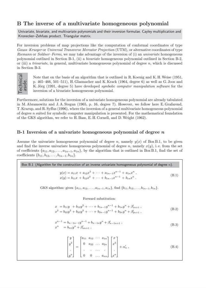
Assume the univariate homogeneous polynomial of degree n, namely y(x) of Box B.1, to be given
and find the inverse univariate homogeneous polynomial of degree n, namely x(y), i. e. from the set
of coefficients {a 11 , a 12 , . . . , a 1n−1 , a 1n }, by the algorithm that is outlined in Box B.1, find the set of
coefficients {b 11 , b 12 , . . . , b 1n−1 , b 1n }.
Box B.1 (Algorithm for the construction of an inverse univariate homogeneous polynomial of degree n).
y(x) = a 11 x + a 12 x
2 + · · · + a 1n−1 x
n−1 + a 1n x
n ,
x(y) = b 11 x + b 12 x
2 + · · · + b 1n−1 x
n−1 + b 1n x
n .
(B.1)
GKS algorithm: given {a 11 , a 12 , . . . , a 1n−1 , a 1n }, find {b 11 , b 12 , . . . , b 1n−1 , b 1n }.
Forward substitution:
x = b 11 y + b 12 y
2 + · · · + b 1n−1 y
n−1 + b 1n y
n + β
1n+1 ,
x
2 = b 22 y
2 + b 23 y
3 + · · · + b 2n−1 y
n−1 + b 2n y
n + β
2n+1 ,
(B.2)
x
n−1 = b n−1n−1 y
n−1 + b n−1n y
n + β
n−1n+1 ,
x
n
= b nn y
n + β
nn+1 ,
(B.3)
2
6
6
6
6
4
y
y
2
.
y
n
3
7
7
7
7
5
=
2
6
6
6
6
4
a 11 a 12 · · · a 1n
0 a 22 . . . a 2n
.
. ... .
0
0 . . . a nn
3
7
7
7
7
5
2
6
6
6
6
4
x
x
2
.
x
n
3
7
7
7
7
5
+ α
n ,
(B.4)
Univariate, bivariate, and multivariate polynomials and their inversion formulae. Cayley multiplication and
Kronecker–Zehfuss product. Triangular matrix.
For inversion problems of map projections like the computation of conformal coordinates of type
Gauss–Krueger or Universal Transverse Mercator Projection (UTM), or alternative coordinates of type
Riemann or Soldner–Fermi, we may take advantage of the inversion of (i) an univariate homogeneous
polynomial outlined in Section B-1, (ii) a bivariate homogeneous polynomial outlined in Section B-2,
or (iii) a trivariate, in general, multivariate homogeneous polynomial of degree n, which is discussed
in Section B-3.
Technical
aside.
Note that on the basis of an algorithm that is outlined in R. Koenig and K. H. Weise (1951,
p. 465–466, 501–511), H. Glasmacher and K. Krack (1964, degree 6) as well as G. Joos and
K. J¨ org (1991, degree 5) have developed symbolic computer manipulation software for the
inversion of a bivariate homogeneous polynomial.
Furthermore, solutions for the inversion of a univariate homogeneous polynomial are already tabulated
in M. Abramowitz and J. A. Stegun (1965, p. 16, degree 7). However, we follow here E. Grafarend,
T. Krarup, and R. Syffus (1996), where the inversion of a general multivariate homogeneous polynomial
of degree n suited for symbolic computer manipulation is presented. For the mathematical foundation
of the GKS algorithm, we refer to H. Bass, E. H. Cornell, and D. Wright (1962).
B-1 Inversion of a univariate homogeneous polynomial of degree n
Assume the univariate homogeneous polynomial of degree n, namely y(x) of Box B.1, to be given
and find the inverse univariate homogeneous polynomial of degree n, namely x(y), i. e. from the set
of coefficients {a 11 , a 12 , . . . , a 1n−1 , a 1n }, by the algorithm that is outlined in Box B.1, find the set of
coefficients {b 11 , b 12 , . . . , b 1n−1 , b 1n }.
Box B.1 (Algorithm for the construction of an inverse univariate homogeneous polynomial of degree n).
y(x) = a 11 x + a 12 x
2 + · · · + a 1n−1 x
n−1 + a 1n x
n ,
x(y) = b 11 x + b 12 x
2 + · · · + b 1n−1 x
n−1 + b 1n x
n .
(B.1)
GKS algorithm: given {a 11 , a 12 , . . . , a 1n−1 , a 1n }, find {b 11 , b 12 , . . . , b 1n−1 , b 1n }.
Forward substitution:
x = b 11 y + b 12 y
2 + · · · + b 1n−1 y
n−1 + b 1n y
n + β
1n+1 ,
x
2 = b 22 y
2 + b 23 y
3 + · · · + b 2n−1 y
n−1 + b 2n y
n + β
2n+1 ,
(B.2)
x
n−1 = b n−1n−1 y
n−1 + b n−1n y
n + β
n−1n+1 ,
x
n
= b nn y
n + β
nn+1 ,
(B.3)
2
6
6
6
6
4
y
y
2
.
y
n
3
7
7
7
7
5
=
2
6
6
6
6
4
a 11 a 12 · · · a 1n
0 a 22 . . . a 2n
.
. ... .
0
0 . . . a nn
3
7
7
7
7
5
2
6
6
6
6
4
x
x
2
.
x
n
3
7
7
7
7
5
+ α
n ,
(B.4)