

492 21 Datum problems
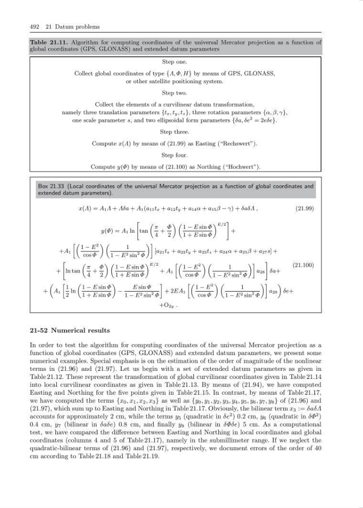
Table 21.11. Algorithm for computing coordinates of the universal Mercator projection as a function of
global coordinates (GPS, GLONASS) and extended datum parameters
Step one.
Collect global coordinates of type {Λ, Φ, H} by means of GPS, GLONASS,
or other satellite positioning system.
Step two.
Collect the elements of a curvilinear datum transformation,
namely three translation parameters {t x , t y , t z }, three rotation parameters {α, β, γ},
one scale parameter s, and two ellipsoidal form parameters {δa, δe
2 = 2eδe}.
Step three.
Compute x(Λ) by means of (21.99) as Easting (“Rechswert”).
Step four.
Compute y(Φ) by means of (21.100) as Northing (“Hochwert”).
Box 21.33 (Local coordinates of the universal Mercator projection as a function of global coordinates and
extended datum parameters).
x(Λ) = A 1 Λ + Λδa + A 1 (a 11 t x + a 12 t y + a 14 α + a 15 β − γ) + δaδΛ ,
(21.99)
y(Φ) = A 1 ln
"
tan
„
π
4
+
Φ
2
« „
1 − E sin Φ
1 + E sin Φ
« E/2
#
+
+A 1
»„
1 − E
2
cos Φ
« „
1
1 − E 2 sin
2 Φ
«–
[a 21 t x + a 22 t y + a 23 t z + a 24 α + a 25 β + a 27 s] +
+
"
ln tan
„
π
4
+
Φ
2
« „
1 − E sin Φ
1 + E sin Φ
« E/2
+ A 1
»„
1 − E
2
cos Φ
« „
1
1 − E 2 sin
2 Φ
«–
a 28
#
δa+
+
„
A 1
»
1
2
ln
„
1 − E sin Φ
1 + E sin Φ
«
−
E sin Φ
1 − E 2 sin
2 Φ
–
+ 2EA 1
»„
1 − E
2
cos Φ
« „
1
1 − E 2 sin
2 Φ
«–
a 29
«
δe+
+O 2y .
(21.100)
21-52 Numerical results
In order to test the algorithm for computing coordinates of the universal Mercator projection as a
function of global coordinates (GPS, GLONASS) and extended datum parameters, we present some
numerical examples. Special emphasis is on the estimation of the order of magnitude of the nonlinear
terms in (21.96) and (21.97). Let us begin with a set of extended datum parameters as given in
Table 21.12. These represent the transformation of global curvilinear coordinates given in Table 21.14
into local curvilinear coordinates as given in Table 21.13. By means of (21.94), we have computed
Easting and Northing for the five points given in Table 21.15. In contrast, by means of Table 21.17,
we have computed the terms {x 0 , x 1 , x 2 , x 3 } as well as {y 0 , y 1 , y 2 , y 3 , y 4 , y 5 , y 6 , y 7 , y 8 } of (21.96) and
(21.97), which sum up to Easting and Northing in Table 21.17. Obviously, the bilinear term x 3 := δaδΛ
accounts for approximately 2 cm, while the terms y 5 (quadratic in δe
2 ) 0.2 cm, y 6 (quadratic in δΦ
2 )
0.4 cm, y 7 (bilinear in δaδe) 0.8 cm, and finally y 8 (bilinear in δΦδe) 5 cm. As a computational
test, we have compared the difference between Easting and Northing in local coordinates and global
coordinates (columns 4 and 5 of Table 21.17), namely in the submillimeter range. If we neglect the
quadratic-bilinear terms of (21.96) and (21.97), respectively, we document errors of the order of 40
cm according to Table 21.18 and Table 21.19.
Table 21.11. Algorithm for computing coordinates of the universal Mercator projection as a function of
global coordinates (GPS, GLONASS) and extended datum parameters
Step one.
Collect global coordinates of type {Λ, Φ, H} by means of GPS, GLONASS,
or other satellite positioning system.
Step two.
Collect the elements of a curvilinear datum transformation,
namely three translation parameters {t x , t y , t z }, three rotation parameters {α, β, γ},
one scale parameter s, and two ellipsoidal form parameters {δa, δe
2 = 2eδe}.
Step three.
Compute x(Λ) by means of (21.99) as Easting (“Rechswert”).
Step four.
Compute y(Φ) by means of (21.100) as Northing (“Hochwert”).
Box 21.33 (Local coordinates of the universal Mercator projection as a function of global coordinates and
extended datum parameters).
x(Λ) = A 1 Λ + Λδa + A 1 (a 11 t x + a 12 t y + a 14 α + a 15 β − γ) + δaδΛ ,
(21.99)
y(Φ) = A 1 ln
"
tan
„
π
4
+
Φ
2
« „
1 − E sin Φ
1 + E sin Φ
« E/2
#
+
+A 1
»„
1 − E
2
cos Φ
« „
1
1 − E 2 sin
2 Φ
«–
[a 21 t x + a 22 t y + a 23 t z + a 24 α + a 25 β + a 27 s] +
+
"
ln tan
„
π
4
+
Φ
2
« „
1 − E sin Φ
1 + E sin Φ
« E/2
+ A 1
»„
1 − E
2
cos Φ
« „
1
1 − E 2 sin
2 Φ
«–
a 28
#
δa+
+
„
A 1
»
1
2
ln
„
1 − E sin Φ
1 + E sin Φ
«
−
E sin Φ
1 − E 2 sin
2 Φ
–
+ 2EA 1
»„
1 − E
2
cos Φ
« „
1
1 − E 2 sin
2 Φ
«–
a 29
«
δe+
+O 2y .
(21.100)
21-52 Numerical results
In order to test the algorithm for computing coordinates of the universal Mercator projection as a
function of global coordinates (GPS, GLONASS) and extended datum parameters, we present some
numerical examples. Special emphasis is on the estimation of the order of magnitude of the nonlinear
terms in (21.96) and (21.97). Let us begin with a set of extended datum parameters as given in
Table 21.12. These represent the transformation of global curvilinear coordinates given in Table 21.14
into local curvilinear coordinates as given in Table 21.13. By means of (21.94), we have computed
Easting and Northing for the five points given in Table 21.15. In contrast, by means of Table 21.17,
we have computed the terms {x 0 , x 1 , x 2 , x 3 } as well as {y 0 , y 1 , y 2 , y 3 , y 4 , y 5 , y 6 , y 7 , y 8 } of (21.96) and
(21.97), which sum up to Easting and Northing in Table 21.17. Obviously, the bilinear term x 3 := δaδΛ
accounts for approximately 2 cm, while the terms y 5 (quadratic in δe
2 ) 0.2 cm, y 6 (quadratic in δΦ
2 )
0.4 cm, y 7 (bilinear in δaδe) 0.8 cm, and finally y 8 (bilinear in δΦδe) 5 cm. As a computational
test, we have compared the difference between Easting and Northing in local coordinates and global
coordinates (columns 4 and 5 of Table 21.17), namely in the submillimeter range. If we neglect the
quadratic-bilinear terms of (21.96) and (21.97), respectively, we document errors of the order of 40
cm according to Table 21.18 and Table 21.19.