

21-3 Error propagation in analysis and synthesis of a datum problem 467
21-3 Error propagation in analysis and synthesis of a datum problem
Nonlinear error propagation. Dispersion, dispersion transformation, dispersion matrix, variance–covariance
matrix. Stochastic pseudo-observations.
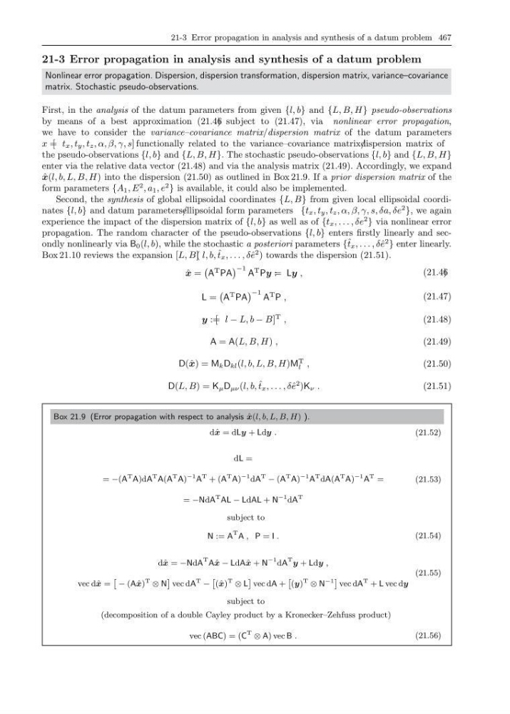
First, in the analysis of the datum parameters from given {l, b} and {L, B, H} pseudo-observations
by means of a best approximation (21.46 ) subject to (21.47), via nonlinear error propagation,
we have to consider the variance–covariance matrix/dispersion matrix of the datum parameters
x = [ t x , t y , t z , α, β, γ, s] functionally related to the variance–covariance matrix/ dispersion matrix of
the pseudo-observations {l, b} and {L, B, H}. The stochastic pseudo-observations {l, b} and {L, B, H}
enter via the relative data vector (21.48) and via the analysis matrix (21.49). Accordingly, we expand
ˆ
x(l, b, L, B, H) into the dispersion (21.50) as outlined in Box 21.9. If a prior dispersion matrix of the
form parameters {A 1 , E
2 , a 1 , e
2
} is available, it could also be implemented.
Second, the synthesis of global ellipsoidal coordinates {L, B} from given local ellipsoidal coordinates {l, b} and datum parameters/ ellipsoidal form parameters {t x , t y , t z , α, β, γ, s, δa, δe
2
}, we again
experience the impact of the dispersion matrix of {l, b} as well as of {t x , . . . , δe
2
} via nonlinear error
propagation. The random character of the pseudo-observations {l, b} enters firstly linearly and secondly nonlinearly via B 0 (l, b), while the stochastic a posteriori parameters { ˆ
t x , . . . , δˆ e
2
} enter linearly.
Box 21.10 reviews the expansion [L, B] ( l, b, ˆ
t x , . . . , δˆ e
2 ) towards the dispersion (21.51).
ˆ
x =
A
T PA
−1 A
T Py = : Ly ,
(21.46 )
L =
A
T PA
−1 A
T P ,
(21.47)
y := [ l − L, b − B]
T ,
(21.48)
A = A(L, B, H) ,
(21.49)
D(ˆ x) = M k D kl (l, b, L, B, H)M
T
l ,
(21.50)
D(L, B) = K µ D µν (l, b, ˆ
t x , . . . , δˆ e
2 )K ν .
(21.51)
Box 21.9 (Error propagation with respect to analysis ˆ
x(l, b, L, B, H) ).
dˆ x = dLy + Ldy .
(21.52)
dL =
= −(A
T A)dA
T A(A
T A)
−1 A
T + (A
T A)
−1 dA
T − (A
T A)
−1 A
T dA(A
T A)
−1 A
T =
= −NdA
T AL − LdAL + N
−1 dA
T
(21.53)
subject to
N := A
T A , P = I .
(21.54)
dˆ x = −NdA
T Aˆ x − LdAˆ x + N
−1 dA
T y + Ldy ,
vec dˆ x =
ˆ − (Aˆ x)
T ⊗ N
˜
vec dA
T −
ˆ
(ˆ x)
T ⊗ L
˜
vec dA +
ˆ
(y)
T ⊗ N
−1
˜
vec dA
T + L vec dy
(21.55)
subject to
(decomposition of a double Cayley product by a Kronecker–Zehfuss product)
vec (ABC) = (C
T ⊗ A) vec B .
(21.56)
21-3 Error propagation in analysis and synthesis of a datum problem
Nonlinear error propagation. Dispersion, dispersion transformation, dispersion matrix, variance–covariance
matrix. Stochastic pseudo-observations.
First, in the analysis of the datum parameters from given {l, b} and {L, B, H} pseudo-observations
by means of a best approximation (21.46 ) subject to (21.47), via nonlinear error propagation,
we have to consider the variance–covariance matrix/dispersion matrix of the datum parameters
x = [ t x , t y , t z , α, β, γ, s] functionally related to the variance–covariance matrix/ dispersion matrix of
the pseudo-observations {l, b} and {L, B, H}. The stochastic pseudo-observations {l, b} and {L, B, H}
enter via the relative data vector (21.48) and via the analysis matrix (21.49). Accordingly, we expand
ˆ
x(l, b, L, B, H) into the dispersion (21.50) as outlined in Box 21.9. If a prior dispersion matrix of the
form parameters {A 1 , E
2 , a 1 , e
2
} is available, it could also be implemented.
Second, the synthesis of global ellipsoidal coordinates {L, B} from given local ellipsoidal coordinates {l, b} and datum parameters/ ellipsoidal form parameters {t x , t y , t z , α, β, γ, s, δa, δe
2
}, we again
experience the impact of the dispersion matrix of {l, b} as well as of {t x , . . . , δe
2
} via nonlinear error
propagation. The random character of the pseudo-observations {l, b} enters firstly linearly and secondly nonlinearly via B 0 (l, b), while the stochastic a posteriori parameters { ˆ
t x , . . . , δˆ e
2
} enter linearly.
Box 21.10 reviews the expansion [L, B] ( l, b, ˆ
t x , . . . , δˆ e
2 ) towards the dispersion (21.51).
ˆ
x =
A
T PA
−1 A
T Py = : Ly ,
(21.46 )
L =
A
T PA
−1 A
T P ,
(21.47)
y := [ l − L, b − B]
T ,
(21.48)
A = A(L, B, H) ,
(21.49)
D(ˆ x) = M k D kl (l, b, L, B, H)M
T
l ,
(21.50)
D(L, B) = K µ D µν (l, b, ˆ
t x , . . . , δˆ e
2 )K ν .
(21.51)
Box 21.9 (Error propagation with respect to analysis ˆ
x(l, b, L, B, H) ).
dˆ x = dLy + Ldy .
(21.52)
dL =
= −(A
T A)dA
T A(A
T A)
−1 A
T + (A
T A)
−1 dA
T − (A
T A)
−1 A
T dA(A
T A)
−1 A
T =
= −NdA
T AL − LdAL + N
−1 dA
T
(21.53)
subject to
N := A
T A , P = I .
(21.54)
dˆ x = −NdA
T Aˆ x − LdAˆ x + N
−1 dA
T y + Ldy ,
vec dˆ x =
ˆ − (Aˆ x)
T ⊗ N
˜
vec dA
T −
ˆ
(ˆ x)
T ⊗ L
˜
vec dA +
ˆ
(y)
T ⊗ N
−1
˜
vec dA
T + L vec dy
(21.55)
subject to
(decomposition of a double Cayley product by a Kronecker–Zehfuss product)
vec (ABC) = (C
T ⊗ A) vec B .
(21.56)