

460 21 Datum problems
Various remarks with respect to the rank and the stability of the Jacobi matrix A have to be
made. First, the Jacobi matrix A indicates that columns seven and eight, namely a 7 and a 8 , are
linearly dependent, in particular, Aa 8 = a 7 . Obviously, the incremental scale s and the incremental
semi-major axis δA cannot be determined independently. Since we cannot discriminate s and δA, we
may consult data files of the global and local reference ellipsoid in order to fix the values δA := A − a
as well as δE
2 := E
2
− e
2 and remove by b − B − (a 28 δA + a 29 δE
2 ) the quantities {δA, δE
2
} from
the analysis. Note that only the differences in latitude are influenced by {s, δA, δE
2
}, respectively.
Second, for a geodetic network for which both {l, b} and {L, B, H} are available, the extension in
latitude {b, B} may lead to an instability within the Jacobi matrix A as we have experienced. In the
analysis of column a 3 (acting on translation component t z ) and column a 7 (acting on scale s), sin B
is approximately discriminating the two columns. In the above-quoted network configuration, a 3 and
a 7 are nearly linearly dependent. The following rationale has accordingly been chosen, following the
method of partial least squares (P. J. Young (1994)), for instance.
Important!
The system (21.23) of linear equations y = Ax + hit is characterized by two pseudo-observed
ellipsoidal longitude and ellipsoidal latitude differences. In case we have access to the ellipsoidal form parameter variation δA and δE
2 , we are left with two equations for seven datum
parameters per station point. Obviously, in order to determine the seven datum parameters,
we need at least four station points with the data {l, b} and {L, B, H} available. But, in
general, we are left with an adjustment problem when the data are accessible at four or
more station points. Since ellipsoidal longitude and ellipsoidal latitude {l, b} are elements
of E
2
a 1 ,a 2
, the distance between the adjusted points and the given data points {l, b} has to
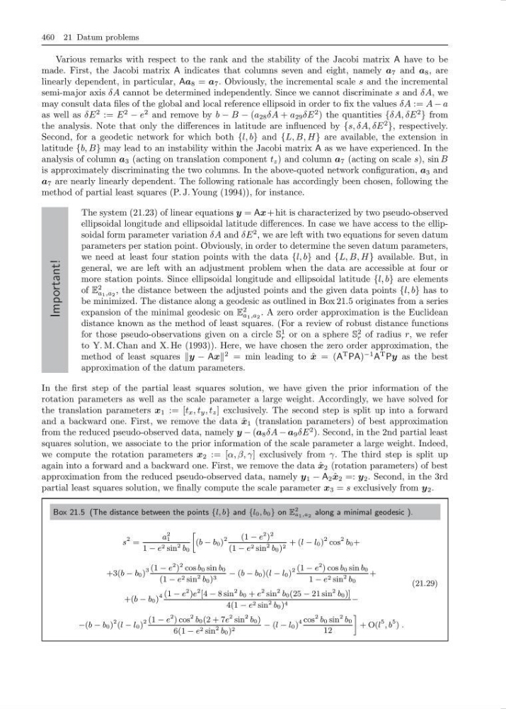
be minimized. The distance along a geodesic as outlined in Box 21.5 originates from a series
expansion of the minimal geodesic on E
2
a 1 ,a 2 . A zero order approximation is the Euclidean
distance known as the method of least squares. (For a review of robust distance functions
for those pseudo-observations given on a circle S
1
r or on a sphere S
2
r of radius r, we refer
to Y. M. Chan and X. He (1993)). Here, we have chosen the zero order approximation, the
method of least squares y − Ax
2 = min leading to ˆ
x = (A
T PA)
−1 A
T Py as the best
approximation of the datum parameters.
In the first step of the partial least squares solution, we have given the prior information of the
rotation parameters as well as the scale parameter a large weight. Accordingly, we have solved for
the translation parameters x 1 := [t x , t y , t z ] exclusively. The second step is split up into a forward
and a backward one. First, we remove the data ˆ
x 1 (translation parameters) of best approximation
from the reduced pseudo-observed data, namely y − (a 8 δA − a 9 δE
2 ). Second, in the 2nd partial least
squares solution, we associate to the prior information of the scale parameter a large weight. Indeed,
we compute the rotation parameters x 2 := [α, β, γ] exclusively from γ. The third step is split up
again into a forward and a backward one. First, we remove the data ˆ
x 2 (rotation parameters) of best
approximation from the reduced pseudo-observed data, namely y 1 − A 2 ˆ
x 2 =: y 2 . Second, in the 3rd
partial least squares solution, we finally compute the scale parameter x 3 = s exclusively from y 2 .
Box 21.5 (The distance between the points {l, b} and {l 0 , b 0 } on E
2
a 1 ,a 2 along a minimal geodesic ).
s
2 =
a
2
1
1 − e 2 sin
2 b 0
»
(b − b 0 )
2
(1 − e
2 )
2
(1 − e 2 sin
2 b 0 ) 2 + (l − l 0 )
2 cos
2 b 0 +
+3(b − b 0 )
3 (1 − e
2 )
2 cos b 0 sin b 0
(1 − e 2 sin
2 b 0 ) 3 − (b − b 0 )(l − l 0 )
2 (1 − e
2 ) cos b 0 sin b 0
1 − e 2 sin
2 b 0
+
+(b − b 0 )
4 (1 − e
2 )e
2 [4 − 8 sin
2 b 0 + e
2 sin
2 b 0 (25 − 21 sin
2 b 0 )]
4(1 − e 2 sin
2 b 0 ) 4
−
−(b − b 0 )
2 (l − l 0 )
2 (1 − e
2 ) cos
2 b 0 (2 + 7e
2 sin
2 b 0 )
6(1 − e 2 sin
2 b 0 ) 2
− (l − l 0 )
4 cos
2 b 0 sin
2 b 0
12
–
+ O(l
5 , b
5 ) .
(21.29)
Various remarks with respect to the rank and the stability of the Jacobi matrix A have to be
made. First, the Jacobi matrix A indicates that columns seven and eight, namely a 7 and a 8 , are
linearly dependent, in particular, Aa 8 = a 7 . Obviously, the incremental scale s and the incremental
semi-major axis δA cannot be determined independently. Since we cannot discriminate s and δA, we
may consult data files of the global and local reference ellipsoid in order to fix the values δA := A − a
as well as δE
2 := E
2
− e
2 and remove by b − B − (a 28 δA + a 29 δE
2 ) the quantities {δA, δE
2
} from
the analysis. Note that only the differences in latitude are influenced by {s, δA, δE
2
}, respectively.
Second, for a geodetic network for which both {l, b} and {L, B, H} are available, the extension in
latitude {b, B} may lead to an instability within the Jacobi matrix A as we have experienced. In the
analysis of column a 3 (acting on translation component t z ) and column a 7 (acting on scale s), sin B
is approximately discriminating the two columns. In the above-quoted network configuration, a 3 and
a 7 are nearly linearly dependent. The following rationale has accordingly been chosen, following the
method of partial least squares (P. J. Young (1994)), for instance.
Important!
The system (21.23) of linear equations y = Ax + hit is characterized by two pseudo-observed
ellipsoidal longitude and ellipsoidal latitude differences. In case we have access to the ellipsoidal form parameter variation δA and δE
2 , we are left with two equations for seven datum
parameters per station point. Obviously, in order to determine the seven datum parameters,
we need at least four station points with the data {l, b} and {L, B, H} available. But, in
general, we are left with an adjustment problem when the data are accessible at four or
more station points. Since ellipsoidal longitude and ellipsoidal latitude {l, b} are elements
of E
2
a 1 ,a 2
, the distance between the adjusted points and the given data points {l, b} has to
be minimized. The distance along a geodesic as outlined in Box 21.5 originates from a series
expansion of the minimal geodesic on E
2
a 1 ,a 2 . A zero order approximation is the Euclidean
distance known as the method of least squares. (For a review of robust distance functions
for those pseudo-observations given on a circle S
1
r or on a sphere S
2
r of radius r, we refer
to Y. M. Chan and X. He (1993)). Here, we have chosen the zero order approximation, the
method of least squares y − Ax
2 = min leading to ˆ
x = (A
T PA)
−1 A
T Py as the best
approximation of the datum parameters.
In the first step of the partial least squares solution, we have given the prior information of the
rotation parameters as well as the scale parameter a large weight. Accordingly, we have solved for
the translation parameters x 1 := [t x , t y , t z ] exclusively. The second step is split up into a forward
and a backward one. First, we remove the data ˆ
x 1 (translation parameters) of best approximation
from the reduced pseudo-observed data, namely y − (a 8 δA − a 9 δE
2 ). Second, in the 2nd partial least
squares solution, we associate to the prior information of the scale parameter a large weight. Indeed,
we compute the rotation parameters x 2 := [α, β, γ] exclusively from γ. The third step is split up
again into a forward and a backward one. First, we remove the data ˆ
x 2 (rotation parameters) of best
approximation from the reduced pseudo-observed data, namely y 1 − A 2 ˆ
x 2 =: y 2 . Second, in the 3rd
partial least squares solution, we finally compute the scale parameter x 3 = s exclusively from y 2 .
Box 21.5 (The distance between the points {l, b} and {l 0 , b 0 } on E
2
a 1 ,a 2 along a minimal geodesic ).
s
2 =
a
2
1
1 − e 2 sin
2 b 0
»
(b − b 0 )
2
(1 − e
2 )
2
(1 − e 2 sin
2 b 0 ) 2 + (l − l 0 )
2 cos
2 b 0 +
+3(b − b 0 )
3 (1 − e
2 )
2 cos b 0 sin b 0
(1 − e 2 sin
2 b 0 ) 3 − (b − b 0 )(l − l 0 )
2 (1 − e
2 ) cos b 0 sin b 0
1 − e 2 sin
2 b 0
+
+(b − b 0 )
4 (1 − e
2 )e
2 [4 − 8 sin
2 b 0 + e
2 sin
2 b 0 (25 − 21 sin
2 b 0 )]
4(1 − e 2 sin
2 b 0 ) 4
−
−(b − b 0 )
2 (l − l 0 )
2 (1 − e
2 ) cos
2 b 0 (2 + 7e
2 sin
2 b 0 )
6(1 − e 2 sin
2 b 0 ) 2
− (l − l 0 )
4 cos
2 b 0 sin
2 b 0
12
–
+ O(l
5 , b
5 ) .
(21.29)