

456 21 Datum problems
E1
E3
E2
e1
e3
e2
P (L, B, H) = P (l, b, h)
Z
Y
X
x
y
z
L
B
l
H
h
b
E
2
A 1 ,A 2
E
2
a 1 ,a 2
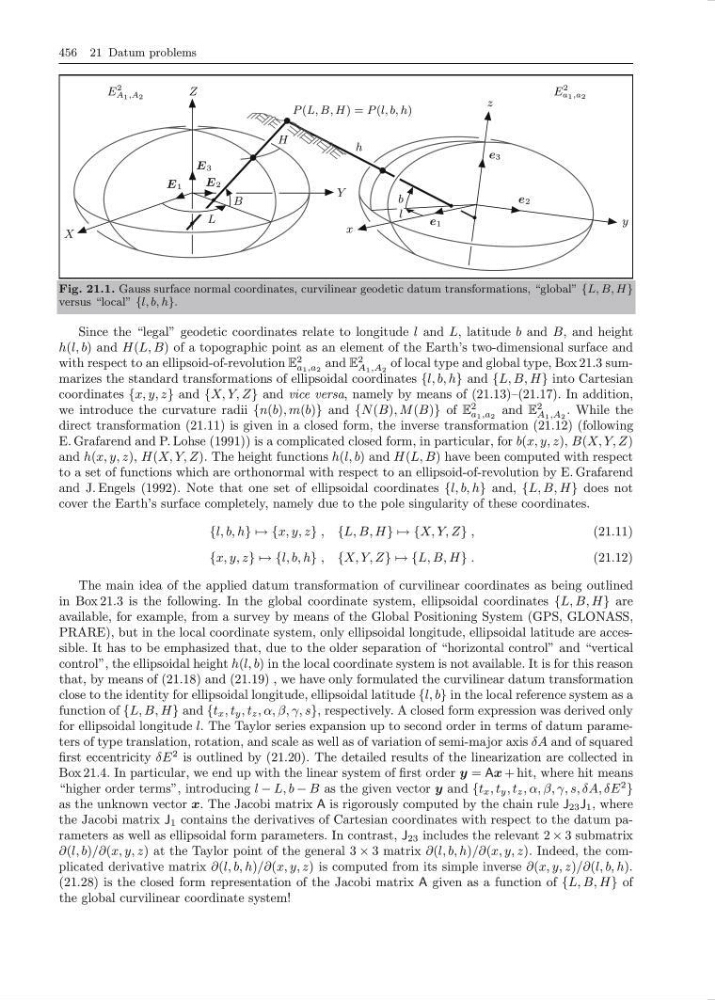
Fig. 21.1. Gauss surface normal coordinates, curvilinear geodetic datum transformations, “global” {L, B, H}
versus “local” {l, b, h}.
Since the “legal” geodetic coordinates relate to longitude l and L, latitude b and B, and height
h(l, b) and H(L, B) of a topographic point as an element of the Earth’s two-dimensional surface and
with respect to an ellipsoid-of-revolution E
2
a 1 ,a 2
and E
2
A 1 ,A 2
of local type and global type, Box 21.3 summarizes the standard transformations of ellipsoidal coordinates {l, b, h} and {L, B, H} into Cartesian
coordinates {x, y, z} and {X, Y, Z} and vice versa, namely by means of (21.13)–(21.17). In addition,
we introduce the curvature radii {n(b), m(b)} and {N (B), M(B)} of E
2
a 1 ,a 2 and E
2
A 1 ,A 2
. While the
direct transformation (21.11) is given in a closed form, the inverse transformation (21.12) (following
E. Grafarend and P. Lohse (1991)) is a complicated closed form, in particular, for b(x, y, z), B(X, Y, Z)
and h(x, y, z), H(X, Y, Z). The height functions h(l, b) and H(L, B) have been computed with respect
to a set of functions which are orthonormal with respect to an ellipsoid-of-revolution by E. Grafarend
and J. Engels (1992). Note that one set of ellipsoidal coordinates {l, b, h} and, {L, B, H} does not
cover the Earth’s surface completely, namely due to the pole singularity of these coordinates.
{l, b, h} → {x, y, z} , {L, B, H} → {X, Y, Z} ,
(21.11)
{x, y, z} → {l, b, h} , {X, Y, Z} → {L, B, H} .
(21.12)
The main idea of the applied datum transformation of curvilinear coordinates as being outlined
in Box 21.3 is the following. In the global coordinate system, ellipsoidal coordinates {L, B, H} are
available, for example, from a survey by means of the Global Positioning System (GPS, GLONASS,
PRARE), but in the local coordinate system, only ellipsoidal longitude, ellipsoidal latitude are accessible. It has to be emphasized that, due to the older separation of “horizontal control” and “vertical
control”, the ellipsoidal height h(l, b) in the local coordinate system is not available. It is for this reason
that, by means of (21.18) and (21.19) , we have only formulated the curvilinear datum transformation
close to the identity for ellipsoidal longitude, ellipsoidal latitude {l, b} in the local reference system as a
function of {L, B, H} and {t x , t y , t z , α, β, γ, s}, respectively. A closed form expression was derived only
for ellipsoidal longitude l. The Taylor series expansion up to second order in terms of datum parameters of type translation, rotation, and scale as well as of variation of semi-major axis δA and of squared
first eccentricity δE
2 is outlined by (21.20). The detailed results of the linearization are collected in
Box 21.4. In particular, we end up with the linear system of first order y = Ax + hit, where hit means
“higher order terms”, introducing l − L, b − B as the given vector y and {t x , t y , t z , α, β, γ, s, δA, δE
2
}
as the unknown vector x. The Jacobi matrix A is rigorously computed by the chain rule J 23 J 1 , where
the Jacobi matrix J 1 contains the derivatives of Cartesian coordinates with respect to the datum parameters as well as ellipsoidal form parameters. In contrast, J 23 includes the relevant 2 × 3 submatrix
∂(l, b)/∂(x, y, z) at the Taylor point of the general 3 × 3 matrix ∂(l, b, h)/∂(x, y, z). Indeed, the complicated derivative matrix ∂(l, b, h)/∂(x, y, z) is computed from its simple inverse ∂(x, y, z)/∂(l, b, h).
(21.28) is the closed form representation of the Jacobi matrix A given as a function of {L, B, H} of
the global curvilinear coordinate system!
E1
E3
E2
e1
e3
e2
P (L, B, H) = P (l, b, h)
Z
Y
X
x
y
z
L
B
l
H
h
b
E
2
A 1 ,A 2
E
2
a 1 ,a 2
Fig. 21.1. Gauss surface normal coordinates, curvilinear geodetic datum transformations, “global” {L, B, H}
versus “local” {l, b, h}.
Since the “legal” geodetic coordinates relate to longitude l and L, latitude b and B, and height
h(l, b) and H(L, B) of a topographic point as an element of the Earth’s two-dimensional surface and
with respect to an ellipsoid-of-revolution E
2
a 1 ,a 2
and E
2
A 1 ,A 2
of local type and global type, Box 21.3 summarizes the standard transformations of ellipsoidal coordinates {l, b, h} and {L, B, H} into Cartesian
coordinates {x, y, z} and {X, Y, Z} and vice versa, namely by means of (21.13)–(21.17). In addition,
we introduce the curvature radii {n(b), m(b)} and {N (B), M(B)} of E
2
a 1 ,a 2 and E
2
A 1 ,A 2
. While the
direct transformation (21.11) is given in a closed form, the inverse transformation (21.12) (following
E. Grafarend and P. Lohse (1991)) is a complicated closed form, in particular, for b(x, y, z), B(X, Y, Z)
and h(x, y, z), H(X, Y, Z). The height functions h(l, b) and H(L, B) have been computed with respect
to a set of functions which are orthonormal with respect to an ellipsoid-of-revolution by E. Grafarend
and J. Engels (1992). Note that one set of ellipsoidal coordinates {l, b, h} and, {L, B, H} does not
cover the Earth’s surface completely, namely due to the pole singularity of these coordinates.
{l, b, h} → {x, y, z} , {L, B, H} → {X, Y, Z} ,
(21.11)
{x, y, z} → {l, b, h} , {X, Y, Z} → {L, B, H} .
(21.12)
The main idea of the applied datum transformation of curvilinear coordinates as being outlined
in Box 21.3 is the following. In the global coordinate system, ellipsoidal coordinates {L, B, H} are
available, for example, from a survey by means of the Global Positioning System (GPS, GLONASS,
PRARE), but in the local coordinate system, only ellipsoidal longitude, ellipsoidal latitude are accessible. It has to be emphasized that, due to the older separation of “horizontal control” and “vertical
control”, the ellipsoidal height h(l, b) in the local coordinate system is not available. It is for this reason
that, by means of (21.18) and (21.19) , we have only formulated the curvilinear datum transformation
close to the identity for ellipsoidal longitude, ellipsoidal latitude {l, b} in the local reference system as a
function of {L, B, H} and {t x , t y , t z , α, β, γ, s}, respectively. A closed form expression was derived only
for ellipsoidal longitude l. The Taylor series expansion up to second order in terms of datum parameters of type translation, rotation, and scale as well as of variation of semi-major axis δA and of squared
first eccentricity δE
2 is outlined by (21.20). The detailed results of the linearization are collected in
Box 21.4. In particular, we end up with the linear system of first order y = Ax + hit, where hit means
“higher order terms”, introducing l − L, b − B as the given vector y and {t x , t y , t z , α, β, γ, s, δA, δE
2
}
as the unknown vector x. The Jacobi matrix A is rigorously computed by the chain rule J 23 J 1 , where
the Jacobi matrix J 1 contains the derivatives of Cartesian coordinates with respect to the datum parameters as well as ellipsoidal form parameters. In contrast, J 23 includes the relevant 2 × 3 submatrix
∂(l, b)/∂(x, y, z) at the Taylor point of the general 3 × 3 matrix ∂(l, b, h)/∂(x, y, z). Indeed, the complicated derivative matrix ∂(l, b, h)/∂(x, y, z) is computed from its simple inverse ∂(x, y, z)/∂(l, b, h).
(21.28) is the closed form representation of the Jacobi matrix A given as a function of {L, B, H} of
the global curvilinear coordinate system!