

20-5 Deformation analysis: Riemann, Soldner, Gauss–Krueger coordinates 443
8
◦
9
◦
10
◦
0
◦
−1
◦
+1
◦
1
8
◦
9
◦
10
◦
48
◦
47
◦
49
◦
1
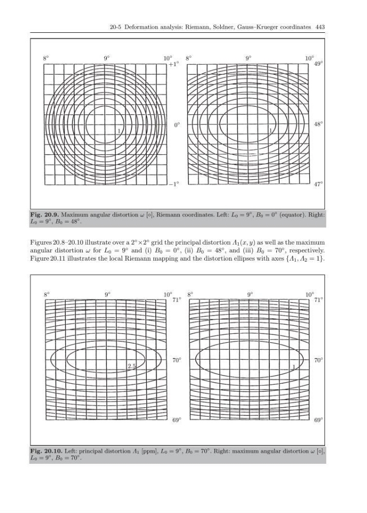
Fig. 20.9. Maximum angular distortion ω [◦], Riemann coordinates. Left: L 0 = 9
◦ , B 0 = 0
◦ (equator). Right:
L 0 = 9
◦ , B 0 = 48
◦ .
Figures 20.8–20.10 illustrate over a 2
◦
×2
◦ grid the principal distortion Λ 1 (x, y) as well as the maximum
angular distortion ω for L 0 = 9
◦ and (i) B 0 = 0
◦ , (ii) B 0 = 48
◦ , and (iii) B 0 = 70
◦ , respectively.
Figure 20.11 illustrates the local Riemann mapping and the distortion ellipses with axes {Λ 1 , Λ 2 = 1}.
8
◦
9
◦
10
◦
70
◦
69
◦
71
◦
2.5
8
◦
9
◦
10
◦
70
◦
69
◦
71
◦
1
Fig. 20.10. Left: principal distortion Λ 1 [ppm], L 0 = 9
◦ , B 0 = 70
◦ . Right: maximum angular distortion ω [◦],
L 0 = 9
◦ , B 0 = 70
◦ .
8
◦
9
◦
10
◦
0
◦
−1
◦
+1
◦
1
8
◦
9
◦
10
◦
48
◦
47
◦
49
◦
1
Fig. 20.9. Maximum angular distortion ω [◦], Riemann coordinates. Left: L 0 = 9
◦ , B 0 = 0
◦ (equator). Right:
L 0 = 9
◦ , B 0 = 48
◦ .
Figures 20.8–20.10 illustrate over a 2
◦
×2
◦ grid the principal distortion Λ 1 (x, y) as well as the maximum
angular distortion ω for L 0 = 9
◦ and (i) B 0 = 0
◦ , (ii) B 0 = 48
◦ , and (iii) B 0 = 70
◦ , respectively.
Figure 20.11 illustrates the local Riemann mapping and the distortion ellipses with axes {Λ 1 , Λ 2 = 1}.
8
◦
9
◦
10
◦
70
◦
69
◦
71
◦
2.5
8
◦
9
◦
10
◦
70
◦
69
◦
71
◦
1
Fig. 20.10. Left: principal distortion Λ 1 [ppm], L 0 = 9
◦ , B 0 = 70
◦ . Right: maximum angular distortion ω [◦],
L 0 = 9
◦ , B 0 = 70
◦ .