

418 20 Geodetic mapping
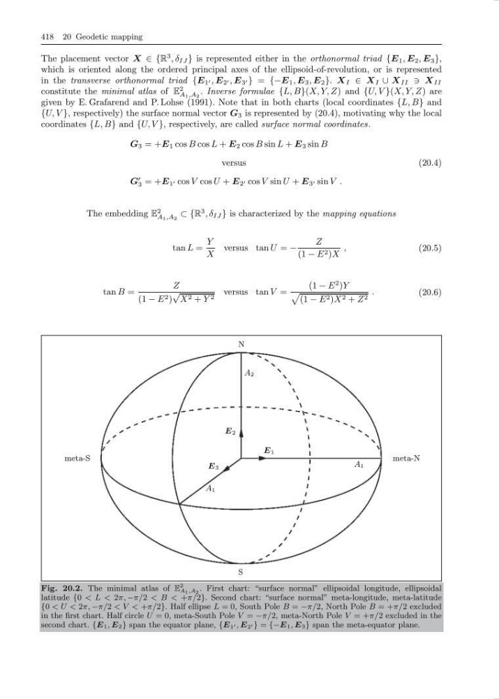
The placement vector X ∈ {R
3 , δ IJ } is represented either in the orthonormal triad {E 1 , E 2 , E 3 },
which is oriented along the ordered principal axes of the ellipsoid-of-revolution, or is represented
in the transverse orthonormal triad {E 1 , E 2 , E 3 } = {−E 1 , E 3 , E 2 }. X I ∈ X I ∪ X II X II
constitute the minimal atlas of E
2
A 1 ,A 2
. Inverse formulae {L, B}(X, Y, Z) and {U, V }(X, Y, Z) are
given by E. Grafarend and P. Lohse (1991). Note that in both charts (local coordinates {L, B} and
{U, V }, respectively) the surface normal vector G 3 is represented by (20.4), motivating why the local
coordinates {L, B} and {U, V }, respectively, are called surface normal coordinates.
G 3 = +E 1 cos B cos L + E 2 cos B sin L + E 3 sin B
versus
G
3 = +E 1 cos V cos U + E 2 cos V sin U + E 3 sin V .
(20.4)
The embedding E
2
A 1 ,A 2
⊂ {R
3 , δ IJ } is characterized by the mapping equations
tan L =
Y
X
versus tan U = −
Z
(1 − E 2 )X
,
(20.5)
tan B =
Z
(1 − E 2 )
√
X 2 + Y 2
versus tan V =
(1 − E
2 )Y
(1 − E 2 )X 2 + Z 2
.
(20.6)
S
N
meta-S
meta-N
A 2
A 1
A 1
E2
E3
E1
Fig. 20.2. The minimal atlas of E
2
A 1 ,A 2 . First chart: “surface normal” ellipsoidal longitude, ellipsoidal
latitude {0 < L < 2π, −π/2 < B < +π/2}. Second chart: “surface normal” meta-longitude, meta-latitude
{0 < U < 2π, −π/2 < V < +π/2}. Half ellipse L = 0, South Pole B = −π/2, North Pole B = +π/2 excluded
in the first chart. Half circle U = 0, meta-South Pole V = −π/2, meta-North Pole V = +π/2 excluded in the
second chart. {E 1 , E 2 } span the equator plane, {E 1 , E 2 } = {−E 1 , E 3 } span the meta-equator plane.
The placement vector X ∈ {R
3 , δ IJ } is represented either in the orthonormal triad {E 1 , E 2 , E 3 },
which is oriented along the ordered principal axes of the ellipsoid-of-revolution, or is represented
in the transverse orthonormal triad {E 1 , E 2 , E 3 } = {−E 1 , E 3 , E 2 }. X I ∈ X I ∪ X II X II
constitute the minimal atlas of E
2
A 1 ,A 2
. Inverse formulae {L, B}(X, Y, Z) and {U, V }(X, Y, Z) are
given by E. Grafarend and P. Lohse (1991). Note that in both charts (local coordinates {L, B} and
{U, V }, respectively) the surface normal vector G 3 is represented by (20.4), motivating why the local
coordinates {L, B} and {U, V }, respectively, are called surface normal coordinates.
G 3 = +E 1 cos B cos L + E 2 cos B sin L + E 3 sin B
versus
G
3 = +E 1 cos V cos U + E 2 cos V sin U + E 3 sin V .
(20.4)
The embedding E
2
A 1 ,A 2
⊂ {R
3 , δ IJ } is characterized by the mapping equations
tan L =
Y
X
versus tan U = −
Z
(1 − E 2 )X
,
(20.5)
tan B =
Z
(1 − E 2 )
√
X 2 + Y 2
versus tan V =
(1 − E
2 )Y
(1 − E 2 )X 2 + Z 2
.
(20.6)
S
N
meta-S
meta-N
A 2
A 1
A 1
E2
E3
E1
Fig. 20.2. The minimal atlas of E
2
A 1 ,A 2 . First chart: “surface normal” ellipsoidal longitude, ellipsoidal
latitude {0 < L < 2π, −π/2 < B < +π/2}. Second chart: “surface normal” meta-longitude, meta-latitude
{0 < U < 2π, −π/2 < V < +π/2}. Half ellipse L = 0, South Pole B = −π/2, North Pole B = +π/2 excluded
in the first chart. Half circle U = 0, meta-South Pole V = −π/2, meta-North Pole V = +π/2 excluded in the
second chart. {E 1 , E 2 } span the equator plane, {E 1 , E 2 } = {−E 1 , E 3 } span the meta-equator plane.