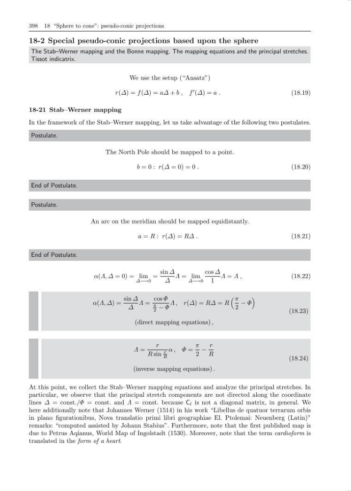
398 18 “Sphere to cone”: pseudo-conic projections
18-2 Special pseudo-conic projections based upon the sphere
The Stab–Werner mapping and the Bonne mapping. The mapping equations and the principal stretches.
Tissot indicatrix.
We use the setup (“Ansatz”)
r(∆) = f (∆) = a∆ + b , f
(∆) = a .
(18.19)
18-21 Stab–Werner mapping
In the framework of the Stab–Werner mapping, let us take advantage of the following two postulates.
Postulate.
The North Pole should be mapped to a point.
b = 0 : r(∆ = 0) = 0 .
(18.20)
End of Postulate.
Postulate.
An arc on the meridian should be mapped equidistantly.
a = R : r(∆) = R∆ .
(18.21)
End of Postulate.
α(Λ, ∆ = 0) = lim
∆−→0
=
sin ∆
∆
Λ = lim
∆−→0
cos ∆
1
Λ = Λ ,
(18.22)
α(Λ, ∆) =
sin ∆
∆
Λ =
cos Φ
π
2 − Φ
Λ , r(∆) = R∆ = R
π
2
− Φ
(direct mapping equations) ,
(18.23)
Λ =
r
R sin
r
R
α , Φ =
π
2
−
r
R
(inverse mapping equations) .
(18.24)
At this point, we collect the Stab–Werner mapping equations and analyze the principal stretches. In
particular, we observe that the principal stretch components are not directed along the coordinate
lines ∆ = const./Φ = const. and Λ = const. because C l is not a diagonal matrix, in general. We
here additionally note that Johannes Werner (1514) in his work “Libellus de quatuor terrarum orbis
in plano figurationibus, Nova translatio primi libri geographiae El. Ptolemai: Neuenberg (Latin)”
remarks: “computed assisted by Johann Stabius”. Furthermore, note that the first published map is
due to Petrus Aqianus, World Map of Ingolstadt (1530). Moreover, note that the term cardioform is
translated in the form of a heart.