388 17 “Sphere to cone”: polar aspect
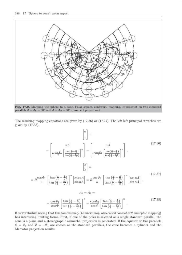
Fig. 17.9. Mapping the sphere to a cone. Polar aspect, conformal mapping, equidistant on two standard
parallels Φ = Φ 0 = 30
◦ and Φ = Φ 0 = 60
◦ (Lambert projection).
The resulting mapping equations are given by (17.36) or (17.37). The left left principal stretches are
given by (17.38).
α
r
=
=
⎡
⎢
⎣
nΛ
R
cos Φ 1
n
tan(
π
4 −
Φ
2 )
tan(
π
4 −
Φ 1
2 )
n
⎤
⎥
⎦ =
⎡
⎢
⎣
nΛ
R
cos Φ 2
n
tan(
π
4 −
Φ
2 )
tan(
π
4 −
Φ 2
2 )
n
⎤
⎥
⎦ ,
(17.36)
x
y
=
= R
cos Φ 1
n
tan
π
4 −
Φ
2
tan
π
4 −
Φ 1
2
n
cos nΛ
sin nΛ
= R
cos Φ 2
n
tan
π
4 −
Φ
2
tan
π
4 −
Φ 2
2
n
cos nΛ
sin nΛ
,
(17.37)
Λ 1 = Λ 2 =
=
cos Φ 1
cos Φ
tan
π
4 −
Φ
2
tan
π
4 −
Φ 1
2
n
=
cos Φ 2
cos Φ
tan
π
4 −
Φ
2
tan
π
4 −
Φ 2
2
n
.
(17.38)
It is worthwhile noting that this famous map (Lambert map, also called conical orthomorphic mapping)
has interesting limiting forms. First, if one of the poles is selected as a single standard parallel, the
cone is a plane and a stereographic azimuthal projection is generated. If the equator or two parallels
Φ = Φ 1 and Φ = −Φ 1 are chosen as the standard parallels, the cone becomes a cylinder and the
Mercator projection results.