

382 17 “Sphere to cone”: polar aspect
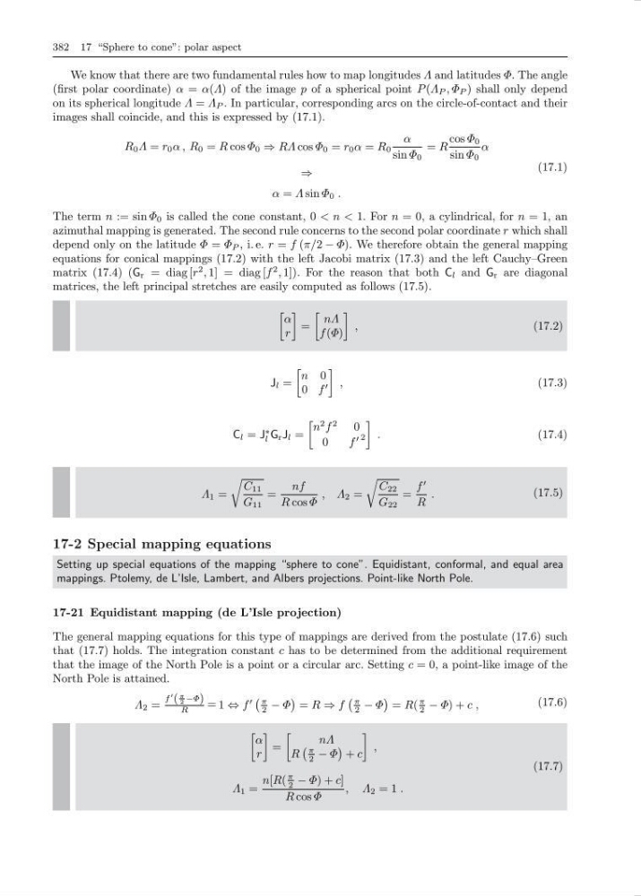
We know that there are two fundamental rules how to map longitudes Λ and latitudes Φ. The angle
(first polar coordinate) α = α(Λ) of the image p of a spherical point P (Λ P , Φ P ) shall only depend
on its spherical longitude Λ = Λ P . In particular, corresponding arcs on the circle-of-contact and their
images shall coincide, and this is expressed by (17.1).
R 0 Λ = r 0 α , R 0 = R cos Φ 0 ⇒ RΛ cos Φ 0 = r 0 α = R 0
α
sin Φ 0
= R
cos Φ 0
sin Φ 0
α
⇒
α = Λ sin Φ 0 .
(17.1)
The term n := sin Φ 0 is called the cone constant, 0 < n < 1. For n = 0, a cylindrical, for n = 1, an
azimuthal mapping is generated. The second rule concerns to the second polar coordinate r which shall
depend only on the latitude Φ = Φ P , i. e. r = f (π/2 − Φ). We therefore obtain the general mapping
equations for conical mappings (17.2) with the left Jacobi matrix (17.3) and the left Cauchy–Green
matrix (17.4) (G r = diag [r
2 , 1] = diag [f
2 , 1]). For the reason that both C l and G r are diagonal
matrices, the left principal stretches are easily computed as follows (17.5).
α
r
=
nΛ
f (Φ)
,
(17.2)
J l =
n 0
0 f
,
(17.3)
C l = J
∗
l G r J l =
n
2 f
2
0
0
f
2
.
(17.4)
Λ 1 =
C 11
G 11
=
nf
R cos Φ
, Λ 2 =
C 22
G 22
=
f
R
.
(17.5)
17-2 Special mapping equations
Setting up special equations of the mapping “sphere to cone”. Equidistant, conformal, and equal area
mappings. Ptolemy, de L’Isle, Lambert, and Albers projections. Point-like North Pole.
17-21 Equidistant mapping (de L’Isle projection)
The general mapping equations for this type of mappings are derived from the postulate (17.6) such
that (17.7) holds. The integration constant c has to be determined from the additional requirement
that the image of the North Pole is a point or a circular arc. Setting c = 0, a point-like image of the
North Pole is attained.
Λ 2 =
f
(
π
2 −Φ)
R
= 1 ⇔ f
π
2 − Φ
= R ⇒ f
π
2 − Φ
= R(
π
2 − Φ) + c ,
(17.6)
α
r
=
nΛ
R
π
2 − Φ
+ c
,
Λ 1 =
n[R(
π
2 − Φ) + c]
R cos Φ
, Λ 2 = 1 .
(17.7)
We know that there are two fundamental rules how to map longitudes Λ and latitudes Φ. The angle
(first polar coordinate) α = α(Λ) of the image p of a spherical point P (Λ P , Φ P ) shall only depend
on its spherical longitude Λ = Λ P . In particular, corresponding arcs on the circle-of-contact and their
images shall coincide, and this is expressed by (17.1).
R 0 Λ = r 0 α , R 0 = R cos Φ 0 ⇒ RΛ cos Φ 0 = r 0 α = R 0
α
sin Φ 0
= R
cos Φ 0
sin Φ 0
α
⇒
α = Λ sin Φ 0 .
(17.1)
The term n := sin Φ 0 is called the cone constant, 0 < n < 1. For n = 0, a cylindrical, for n = 1, an
azimuthal mapping is generated. The second rule concerns to the second polar coordinate r which shall
depend only on the latitude Φ = Φ P , i. e. r = f (π/2 − Φ). We therefore obtain the general mapping
equations for conical mappings (17.2) with the left Jacobi matrix (17.3) and the left Cauchy–Green
matrix (17.4) (G r = diag [r
2 , 1] = diag [f
2 , 1]). For the reason that both C l and G r are diagonal
matrices, the left principal stretches are easily computed as follows (17.5).
α
r
=
nΛ
f (Φ)
,
(17.2)
J l =
n 0
0 f
,
(17.3)
C l = J
∗
l G r J l =
n
2 f
2
0
0
f
2
.
(17.4)
Λ 1 =
C 11
G 11
=
nf
R cos Φ
, Λ 2 =
C 22
G 22
=
f
R
.
(17.5)
17-2 Special mapping equations
Setting up special equations of the mapping “sphere to cone”. Equidistant, conformal, and equal area
mappings. Ptolemy, de L’Isle, Lambert, and Albers projections. Point-like North Pole.
17-21 Equidistant mapping (de L’Isle projection)
The general mapping equations for this type of mappings are derived from the postulate (17.6) such
that (17.7) holds. The integration constant c has to be determined from the additional requirement
that the image of the North Pole is a point or a circular arc. Setting c = 0, a point-like image of the
North Pole is attained.
Λ 2 =
f
(
π
2 −Φ)
R
= 1 ⇔ f
π
2 − Φ
= R ⇒ f
π
2 − Φ
= R(
π
2 − Φ) + c ,
(17.6)
α
r
=
nΛ
R
π
2 − Φ
+ c
,
Λ 1 =
n[R(
π
2 − Φ) + c]
R cos Φ
, Λ 2 = 1 .
(17.7)