

1-3 Two examples: pseudo-cylindrical and orthogonal map projections 23
Fig. 1.10. Orthogonal projection of points of the sphere S
2
R + onto the tangent plane P
2
O at the North Pole,
shorelines, right Tissot ellipses of distorsion.
Example 1.6 (Orthogonal projection of points of the sphere onto the equatorial plane through the origin).
Let us assume that we make an orthogonal projection of points of the northern hemisphere onto the
equatorial plane P
2
O through the origin O of the plane S
2
R + . Figure 1.10 and Figure 1.11 illustrate
such an azimuthal projection by means of polar coordinate lines, shorelines, and right Tissot ellipses
of distortion. The mapping equations are given by x = X, y = Y , Z > 0, x = R cos Φ cos Λ, y =
R cos Φ sin Λ.
End of Example.
e 1
e 2
f α f r
r
α
λ 1
λ 2
ϕ
O
p
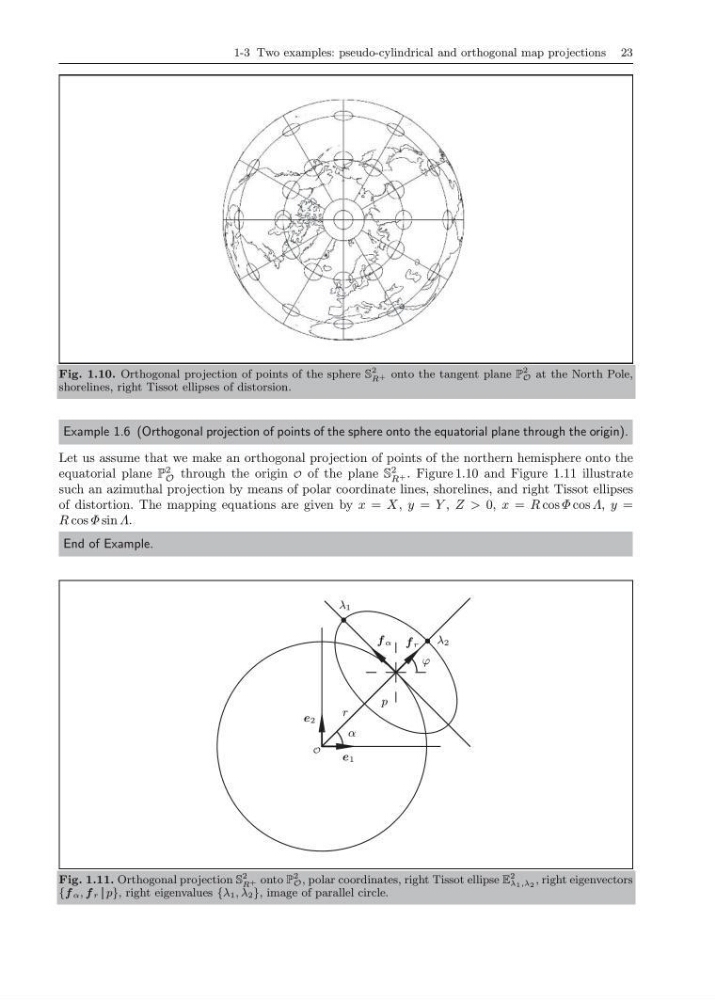
Fig. 1.11. Orthogonal projection S
2
R + onto P
2
O , polar coordinates, right Tissot ellipse E
2
λ 1 ,λ 2 , right eigenvectors
{f α , f r p}, right eigenvalues {λ 1 , λ 2 }, image of parallel circle.
Fig. 1.10. Orthogonal projection of points of the sphere S
2
R + onto the tangent plane P
2
O at the North Pole,
shorelines, right Tissot ellipses of distorsion.
Example 1.6 (Orthogonal projection of points of the sphere onto the equatorial plane through the origin).
Let us assume that we make an orthogonal projection of points of the northern hemisphere onto the
equatorial plane P
2
O through the origin O of the plane S
2
R + . Figure 1.10 and Figure 1.11 illustrate
such an azimuthal projection by means of polar coordinate lines, shorelines, and right Tissot ellipses
of distortion. The mapping equations are given by x = X, y = Y , Z > 0, x = R cos Φ cos Λ, y =
R cos Φ sin Λ.
End of Example.
e 1
e 2
f α f r
r
α
λ 1
λ 2
ϕ
O
p
Fig. 1.11. Orthogonal projection S
2
R + onto P
2
O , polar coordinates, right Tissot ellipse E
2
λ 1 ,λ 2 , right eigenvectors
{f α , f r p}, right eigenvalues {λ 1 , λ 2 }, image of parallel circle.