

16-1 The equations governing conformal mapping 363
Once one system of conformal coordinates is established, we can use it as the input for another system
of conformal coordinates (conformal change from one conformal chart to another conformal chart,
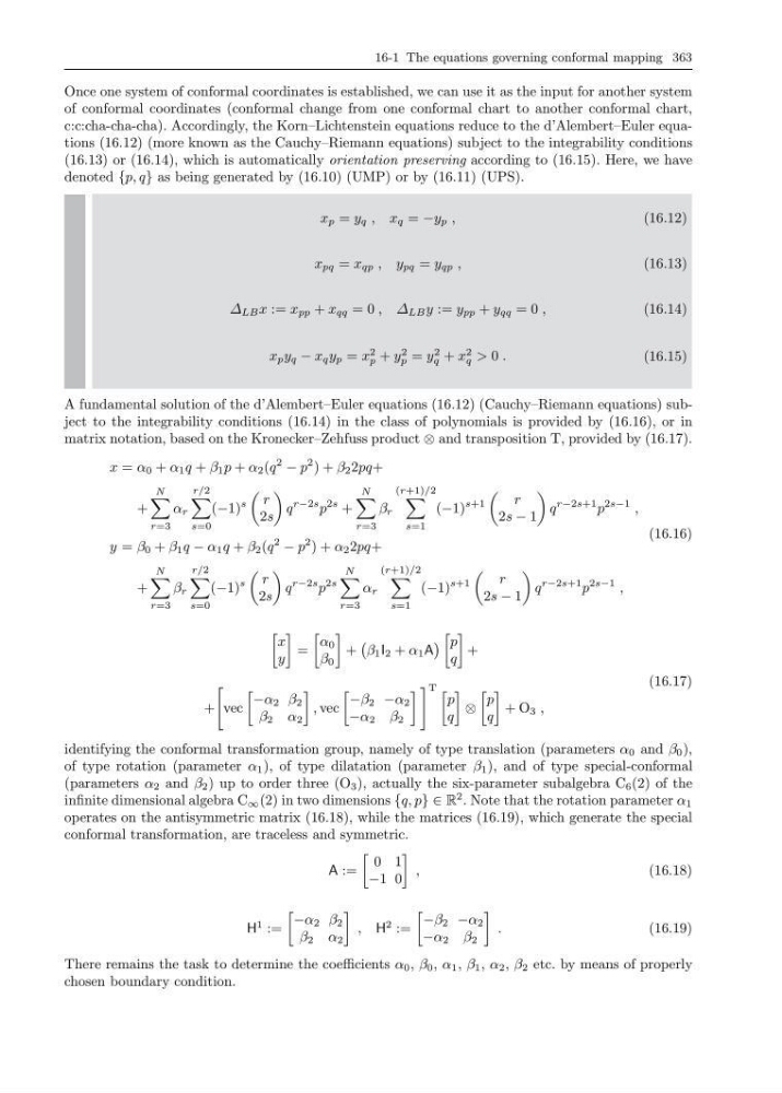
c:c:cha-cha-cha). Accordingly, the Korn–Lichtenstein equations reduce to the d’Alembert–Euler equations (16.12) (more known as the Cauchy–Riemann equations) subject to the integrability conditions
(16.13) or (16.14), which is automatically orientation preserving according to (16.15). Here, we have
denoted {p, q} as being generated by (16.10) (UMP) or by (16.11) (UPS).
x p = y q , x q = −y p ,
(16.12)
x pq = x qp , y pq = y qp ,
(16.13)
∆ LB x := x pp + x qq = 0 , ∆ LB y := y pp + y qq = 0 ,
(16.14)
x p y q − x q y p = x
2
p + y
2
p = y
2
q + x
2
q > 0 .
(16.15)
A fundamental solution of the d’Alembert–Euler equations (16.12) (Cauchy–Riemann equations) subject to the integrability conditions (16.14) in the class of polynomials is provided by (16.16), or in
matrix notation, based on the Kronecker–Zehfuss product ⊗ and transposition T, provided by (16.17).
x = α 0 + α 1 q + β 1 p + α 2 (q
2
− p
2 ) + β 2 2pq+
+
N
r=3
α r
r/2
s=0
(−1)
s
r
2s
q
r−2s p
2s +
N
r=3
β r
(r+1)/2
s=1
(−1)
s+1
r
2s − 1
q
r−2s+1 p
2s−1 ,
y = β 0 + β 1 q − α 1 q + β 2 (q
2
− p
2 ) + α 2 2pq+
+
N
r=3
β r
r/2
s=0
(−1)
s
r
2s
q
r−2s p
2s
N
r=3
α r
(r+1)/2
s=1
(−1)
s+1
r
2s − 1
q
r−2s+1 p
2s−1 ,
(16.16)
x
y
=
α 0
β 0
+
β 1 I 2 + α 1 A
p
q
+
+
vec
−α 2 β 2
β 2 α 2
, vec
−β 2 −α 2
−α 2 β 2
T
p
q
⊗
p
q
+ O 3 ,
(16.17)
identifying the conformal transformation group, namely of type translation (parameters α 0 and β 0 ),
of type rotation (parameter α 1 ), of type dilatation (parameter β 1 ), and of type special-conformal
(parameters α 2 and β 2 ) up to order three (O 3 ), actually the six-parameter subalgebra C 6 (2) of the
infinite dimensional algebra C ∞ (2) in two dimensions {q, p} ∈ R
2 . Note that the rotation parameter α 1
operates on the antisymmetric matrix (16.18), while the matrices (16.19), which generate the special
conformal transformation, are traceless and symmetric.
A :=
0 1
−1 0
,
(16.18)
H
1 :=
−α 2 β 2
β 2 α 2
, H
2 :=
−β 2 −α 2
−α 2 β 2
.
(16.19)
There remains the task to determine the coefficients α 0 , β 0 , α 1 , β 1 , α 2 , β 2 etc. by means of properly
chosen boundary condition.
Once one system of conformal coordinates is established, we can use it as the input for another system
of conformal coordinates (conformal change from one conformal chart to another conformal chart,
c:c:cha-cha-cha). Accordingly, the Korn–Lichtenstein equations reduce to the d’Alembert–Euler equations (16.12) (more known as the Cauchy–Riemann equations) subject to the integrability conditions
(16.13) or (16.14), which is automatically orientation preserving according to (16.15). Here, we have
denoted {p, q} as being generated by (16.10) (UMP) or by (16.11) (UPS).
x p = y q , x q = −y p ,
(16.12)
x pq = x qp , y pq = y qp ,
(16.13)
∆ LB x := x pp + x qq = 0 , ∆ LB y := y pp + y qq = 0 ,
(16.14)
x p y q − x q y p = x
2
p + y
2
p = y
2
q + x
2
q > 0 .
(16.15)
A fundamental solution of the d’Alembert–Euler equations (16.12) (Cauchy–Riemann equations) subject to the integrability conditions (16.14) in the class of polynomials is provided by (16.16), or in
matrix notation, based on the Kronecker–Zehfuss product ⊗ and transposition T, provided by (16.17).
x = α 0 + α 1 q + β 1 p + α 2 (q
2
− p
2 ) + β 2 2pq+
+
N
r=3
α r
r/2
s=0
(−1)
s
r
2s
q
r−2s p
2s +
N
r=3
β r
(r+1)/2
s=1
(−1)
s+1
r
2s − 1
q
r−2s+1 p
2s−1 ,
y = β 0 + β 1 q − α 1 q + β 2 (q
2
− p
2 ) + α 2 2pq+
+
N
r=3
β r
r/2
s=0
(−1)
s
r
2s
q
r−2s p
2s
N
r=3
α r
(r+1)/2
s=1
(−1)
s+1
r
2s − 1
q
r−2s+1 p
2s−1 ,
(16.16)
x
y
=
α 0
β 0
+
β 1 I 2 + α 1 A
p
q
+
+
vec
−α 2 β 2
β 2 α 2
, vec
−β 2 −α 2
−α 2 β 2
T
p
q
⊗
p
q
+ O 3 ,
(16.17)
identifying the conformal transformation group, namely of type translation (parameters α 0 and β 0 ),
of type rotation (parameter α 1 ), of type dilatation (parameter β 1 ), and of type special-conformal
(parameters α 2 and β 2 ) up to order three (O 3 ), actually the six-parameter subalgebra C 6 (2) of the
infinite dimensional algebra C ∞ (2) in two dimensions {q, p} ∈ R
2 . Note that the rotation parameter α 1
operates on the antisymmetric matrix (16.18), while the matrices (16.19), which generate the special
conformal transformation, are traceless and symmetric.
A :=
0 1
−1 0
,
(16.18)
H
1 :=
−α 2 β 2
β 2 α 2
, H
2 :=
−β 2 −α 2
−α 2 β 2
.
(16.19)
There remains the task to determine the coefficients α 0 , β 0 , α 1 , β 1 , α 2 , β 2 etc. by means of properly
chosen boundary condition.