13-2 Special mapping equations 299
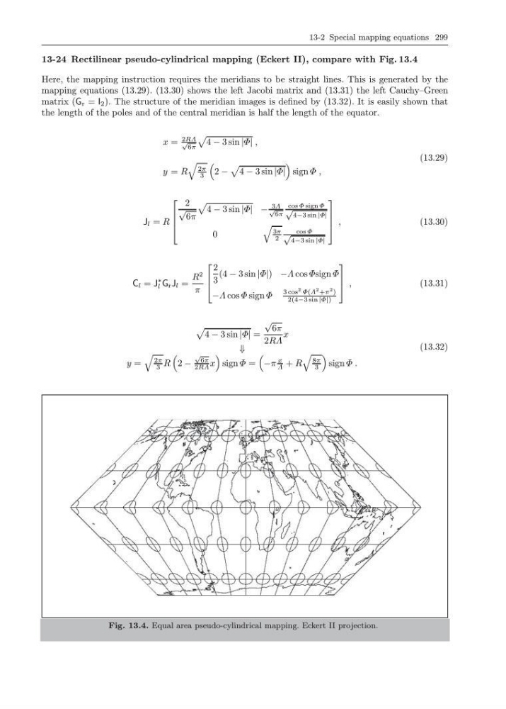
13-24 Rectilinear pseudo-cylindrical mapping (Eckert II), compare with Fig. 13.4
Here, the mapping instruction requires the meridians to be straight lines. This is generated by the
mapping equations (13.29). (13.30) shows the left Jacobi matrix and (13.31) the left Cauchy–Green
matrix (G r = I 2 ). The structure of the meridian images is defined by (13.32). It is easily shown that
the length of the poles and of the central meridian is half the length of the equator.
x =
2RΛ √
6π
4 − 3 sin |Φ| ,
y = R
2π
3
2 −
4 − 3 sin |Φ|
sign Φ ,
(13.29)
J l = R
⎡
⎢
⎢
⎣
2
√
6π
4 − 3 sin |Φ| −
3Λ
√
6π
cos Φ sign Φ
√
4−3 sin |Φ|
0
3π
2
cos Φ
√
4−3 sin |Φ|
⎤
⎥
⎥
⎦ ,
(13.30)
C l = J
∗
l G r J l =
R
2
π
⎡
⎢
⎣
2
3
(4 − 3 sin |Φ|) −Λ cos Φsign Φ
−Λ cos Φ sign Φ
3 cos
2 Φ(Λ
2 +π
2 )
2(4−3 sin |Φ|)
⎤
⎥
⎦ ,
(13.31)
4 − 3 sin |Φ| =
√
6π
2RΛ
x
⇓
y =
2π
3 R
2 −
√
6π
2RΛ x
sign Φ =
−π
x
Λ + R
8π
3
sign Φ .
(13.32)
Fig. 13.4. Equal area pseudo-cylindrical mapping. Eckert II projection.