294 13 “Sphere to cylinder”: pseudo-cylindrical projections
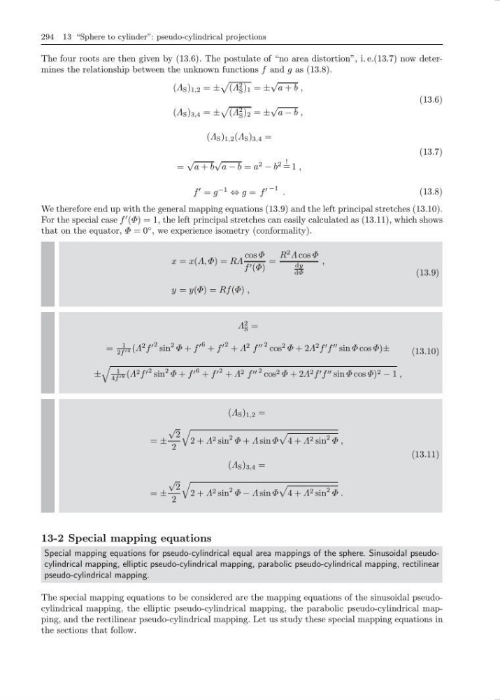
The four roots are then given by (13.6). The postulate of “no area distortion”, i. e.(13.7) now determines the relationship between the unknown functions f and g as (13.8).
(Λ S ) 1,2 = ±
(Λ 2
S ) 1 = ±
√
a + b ,
(Λ S ) 3,4 = ±
(Λ 2
S ) 2 = ±
√
a − b ,
(13.6)
(Λ S ) 1,2 (Λ S ) 3,4 =
=
√
a + b
√
a − b = a
2
− b
2 !
= 1 ,
(13.7)
f
= g
−1
⇔ g = f
−1 .
(13.8)
We therefore end up with the general mapping equations (13.9) and the left principal stretches (13.10).
For the special case f
(Φ) = 1, the left principal stretches can easily calculated as (13.11), which shows
that on the equator, Φ = 0
◦ , we experience isometry (conformality).
x = x(Λ, Φ) = RΛ
cos Φ
f (Φ)
=
R
2 Λ cos Φ
dy
dΦ
,
y = y(Φ) = Rf (Φ) ,
(13.9)
Λ
2
S =
=
1
2f 4 (Λ
2 f
2 sin
2 Φ + f
6 + f
2 + Λ
2 f
2 cos
2 Φ + 2Λ
2 f
f
sin Φ cos Φ)±
±
1
4f 8 (Λ 2 f 2 sin
2 Φ + f 6 + f 2 + Λ 2 f 2 cos 2 Φ + 2Λ 2 f f sin Φ cos Φ) 2 − 1 ,
(13.10)
(Λ S ) 1,2 =
= ±
√
2
2
2 + Λ 2 sin
2 Φ + Λ sin Φ
4 + Λ 2 sin
2 Φ ,
(Λ S ) 3,4 =
= ±
√
2
2
2 + Λ 2 sin
2 Φ − Λ sin Φ
4 + Λ 2 sin
2 Φ .
(13.11)
13-2 Special mapping equations
Special mapping equations for pseudo-cylindrical equal area mappings of the sphere. Sinusoidal pseudocylindrical mapping, elliptic pseudo-cylindrical mapping, parabolic pseudo-cylindrical mapping, rectilinear
pseudo-cylindrical mapping.
The special mapping equations to be considered are the mapping equations of the sinusoidal pseudocylindrical mapping, the elliptic pseudo-cylindrical mapping, the parabolic pseudo-cylindrical mapping, and the rectilinear pseudo-cylindrical mapping. Let us study these special mapping equations in
the sections that follow.