7-2 Special mapping equations 217
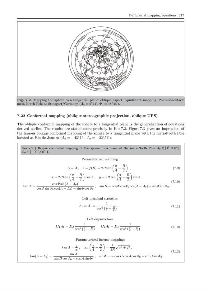
Fig. 7.2. Mapping the sphere to a tangential plane: oblique aspect, equidistant mapping. Point-of-contact:
meta-North Pole at Stuttgart/Germany (Λ 0 = 9
◦ 11
, Φ 0 = 48
◦ 46
).
7-22 Conformal mapping (oblique stereographic projection, oblique UPS)
The oblique conformal mapping of the sphere to a tangential plane is the generalization of equations
derived earlier. The results are stated more precisely in Box 7.2. Figure 7.3 gives an impression of
the famous oblique conformal mapping of the sphere to a tangential plane with the meta-North Pole
located at Rio de Janeiro (Λ 0 = −43
◦ 12
, Φ 0 = −22
◦ 54
).
Box 7.2 (Oblique conformal mapping of the sphere to a plane at the meta-North Pole Λ 0 ∈ [0
◦ , 360
◦ ],
Φ 0 ∈ [−90
◦ , 90
◦ ]).
Parameterized mapping:
α = A , r = f (B) = 2R tan
„
π
4
−
B
2
«
,
(7.9)
x = 2R tan
„
π
4
−
B
2
«
cos A , y = 2R tan
„
π
4
−
B
2
«
sin A ,
tan A =
cos Φ sin(Λ − Λ 0 )
cos Φ sin Φ 0 cos(Λ − Λ 0 ) − sin Φ cos Φ 0
, sin B = cos Φ cos Φ 0 cos(Λ − Λ 0 ) + sin Φ sin Φ 0 .
(7.10)
Left principal stretches:
Λ 1 = Λ 2 =
1
cos 2
` π
4
−
B
2
´ .
(7.11)
Left eigenvectors:
C 1 Λ 1 = E A
1
cos 2
` π
4
−
B
2
´ , C 2 Λ 2 = E B
1
cos 2
` π
4
−
B
2
´ .
(7.12)
Parameterized inverse mapping:
tan A =
y
x
, tan
„
π
4
−
B
2
«
=
1
2R
p
x 2 + y 2 ,
tan(Λ − Λ 0 ) =
sin A
tan B cos Φ 0 + cos A sin Φ 0
, sin Φ = − cos B cos A cos Φ 0 + sin B sin Φ 0 .
(7.13)