

7 “Sphere to tangential plane”: oblique aspect
M
apping the sphere to a tangential plane: meta-azimut hal projections in the oblique aspect. Equidistant,
conformal (oblique UPS), and equal area (oblique Lambert) mappings.
In this chapter, we generalize the concept of azimuthal projections and present the class of widely
applied oblique azimuthal projection. The point-of-contact is not anymore restricted to be one of
the poles or lying on the equator, it can be any point on the reference sphere, i. e. Λ 0 ∈ [0
◦ , 360
◦ ],
Φ 0 ∈ [−90
◦ , 90
◦ ]. With this configuration, any region of interest can be mapped by an equidistant,
conformal, or equal area projection. The latter one is in particular appropriate for regions which
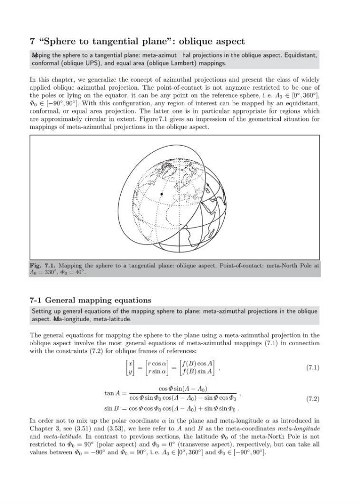
are approximately circular in extent. Figure 7.1 gives an impression of the geometrical situation for
mappings of meta-azimuthal projections in the oblique aspect.
Fig. 7.1. Mapping the sphere to a tangential plane: oblique aspect. Point-of-contact: meta-North Pole at
Λ 0 = 330
◦ , Φ 0 = 40
◦ .
7-1 General mapping equations
Setting up general equations of the mapping sphere to plane: meta-azimuthal projections in the oblique
aspect. M eta-longitude, meta-latitude.
The general equations for mapping the sphere to the plane using a meta-azimuthal projection in the
oblique aspect involve the most general equations of meta-azimuthal mappings (7.1) in connection
with the constraints (7.2) for oblique frames of references:
x
y
=
r cos α
r sin α
=
f (B) cos A
f (B) sin A
,
(7.1)
tan A =
cos Φ sin(Λ − Λ 0 )
cos Φ sin Φ 0 cos(Λ − Λ 0 ) − sin Φ cos Φ 0
,
sin B = cos Φ cos Φ 0 cos(Λ − Λ 0 ) + sin Φ sin Φ 0 .
(7.2)
In order not to mix up the polar coordinate α in the plane and meta-longitude α as introduced in
Chapter 3, see (3.51) and (3.53), we here refer to A and B as the meta-coordinates meta-longitude
and meta-latitude. In contrast to previous sections, the latitude Φ 0 of the meta-North Pole is not
restricted to Φ 0 = 90
◦ (polar aspect) and Φ 0 = 0
◦ (transverse aspect), respectively, but can take all
values between Φ 0 = −90
◦ and Φ 0 = 90
◦ , i. e. Λ 0 ∈ [0
◦ , 360
◦ ] and Φ 0 ∈ [−90
◦ , 90
◦ ].
M
apping the sphere to a tangential plane: meta-azimut hal projections in the oblique aspect. Equidistant,
conformal (oblique UPS), and equal area (oblique Lambert) mappings.
In this chapter, we generalize the concept of azimuthal projections and present the class of widely
applied oblique azimuthal projection. The point-of-contact is not anymore restricted to be one of
the poles or lying on the equator, it can be any point on the reference sphere, i. e. Λ 0 ∈ [0
◦ , 360
◦ ],
Φ 0 ∈ [−90
◦ , 90
◦ ]. With this configuration, any region of interest can be mapped by an equidistant,
conformal, or equal area projection. The latter one is in particular appropriate for regions which
are approximately circular in extent. Figure 7.1 gives an impression of the geometrical situation for
mappings of meta-azimuthal projections in the oblique aspect.
Fig. 7.1. Mapping the sphere to a tangential plane: oblique aspect. Point-of-contact: meta-North Pole at
Λ 0 = 330
◦ , Φ 0 = 40
◦ .
7-1 General mapping equations
Setting up general equations of the mapping sphere to plane: meta-azimuthal projections in the oblique
aspect. M eta-longitude, meta-latitude.
The general equations for mapping the sphere to the plane using a meta-azimuthal projection in the
oblique aspect involve the most general equations of meta-azimuthal mappings (7.1) in connection
with the constraints (7.2) for oblique frames of references:
x
y
=
r cos α
r sin α
=
f (B) cos A
f (B) sin A
,
(7.1)
tan A =
cos Φ sin(Λ − Λ 0 )
cos Φ sin Φ 0 cos(Λ − Λ 0 ) − sin Φ cos Φ 0
,
sin B = cos Φ cos Φ 0 cos(Λ − Λ 0 ) + sin Φ sin Φ 0 .
(7.2)
In order not to mix up the polar coordinate α in the plane and meta-longitude α as introduced in
Chapter 3, see (3.51) and (3.53), we here refer to A and B as the meta-coordinates meta-longitude
and meta-latitude. In contrast to previous sections, the latitude Φ 0 of the meta-North Pole is not
restricted to Φ 0 = 90
◦ (polar aspect) and Φ 0 = 0
◦ (transverse aspect), respectively, but can take all
values between Φ 0 = −90
◦ and Φ 0 = 90
◦ , i. e. Λ 0 ∈ [0
◦ , 360
◦ ] and Φ 0 ∈ [−90
◦ , 90
◦ ].