

200 5 “Sphere to tangential plane”: polar (normal) aspect
Continuation of Box.
(iv) Gnomonic polar azimuthal projection:
J 4 :=
J
2πR 2 =
1
2
Z ∆
0
sin x
1 + cos
2 x
cos 4 x
dx =
1
2
Z ∆
0
sin x
„
1
cos 4 x
+
1
cos 2 x
«
dx ,
J 4 =
1
6
ˆ
1/ cos
3 x
˜ ∆
0
+
1
2
[1/ cos x]
∆
0 ,
J 4 =
1
6
„
1
cos 3 ∆
− 1
«
+
1
2
„
1
cos ∆
− 1
«
,
J 4 =
1
6
1 − cos
3 ∆
cos 3 ∆
+
1
2
1 − cos ∆
cos ∆
.
(5.131)
(v) Orthographic polar azimuthal projection:
J 5 :=
J
2πR 2 =
1
2
Z ∆
0
sin x(1 + cos
2 x)dx , J 5 =
1
2
Z ∆
0
sin xdx +
1
2
Z ∆
0
sin x cos
2 xdx ,
J 5 =
1
2
[− cos x]
∆
0 −
1
6
ˆ
cos
3 x
˜ ∆
0
, J 5 =
1
2
(1 − cos ∆) +
1
6
(1 − cos
3 ∆) .
(5.132)
(vi) Lagrange conformal polar azimuthal projection:
J 6 :=
J
2πR 2 =
1
4
Z ∆
0
sin x
cos 4 x
2
dx =
1
2
Z ∆
0
sin
x
2
cos 3 x
2
dx ,
sin x = 2 sin
x
2
cos
x
2
, x/2 = y : dx = 2dy ,
J 6 =
Z ∆/2
0
sin y
cos 3 y
dy =
1
2
ˆ
1/ cos
2 y
˜ ∆/2
0
=
1
2
1
cos 2 ∆
2
− 1
!
,
J 6 =
1
2
tan
2 ∆
2
.
(5.133)
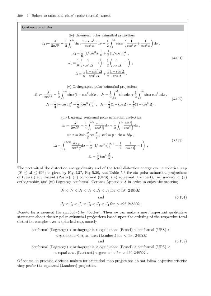
The portrait of the distortion energy density and of the total distortion energy over a spherical cap
(0
◦
≤ ∆ ≤ 60
◦ ) is given by Fig. 5.27, Fig. 5.28, and Table 5.3 for six polar azimuthal projections
of type (i) equidistant (Postel), (ii) conformal (UPS), (iii) equiareal (Lambert), (iv) gnomonic, (v)
orthographic, and (vi) Lagrange conformal. Contact Appendix A in order to enjoy the ordering
J 6 < J 5 < J 1 < J 2 < J 4 < J 3 for < 49
◦ , 248502
and
J 6 < J 5 < J 1 < J 2 < J 3 < J 4 for > 49
◦ , 248502 .
(5.134)
Denote for a moment the symbol < by “better”. Then we can make a most important qualitative
statement about the six polar azimuthal projections based upon the ordering of the respective total
distortion energies over a spherical cap, namely
conformal (Lagrange) < orthographic < equidistant (Postel) < conformal (UPS) <
< gnomonic < equal area (Lambert) for < 49
◦ , 248502
and
conformal (Lagrange) < orthographic < equidistant (Postel) < conformal (UPS) <
< equal area (Lambert) < gnomonic for > 49
◦ , 248502 .
(5.135)
Of course, in practice, decision makers for azimuthal map projections do not follow objective criteria:
they prefer the equiareal (Lambert) projection.
Continuation of Box.
(iv) Gnomonic polar azimuthal projection:
J 4 :=
J
2πR 2 =
1
2
Z ∆
0
sin x
1 + cos
2 x
cos 4 x
dx =
1
2
Z ∆
0
sin x
„
1
cos 4 x
+
1
cos 2 x
«
dx ,
J 4 =
1
6
ˆ
1/ cos
3 x
˜ ∆
0
+
1
2
[1/ cos x]
∆
0 ,
J 4 =
1
6
„
1
cos 3 ∆
− 1
«
+
1
2
„
1
cos ∆
− 1
«
,
J 4 =
1
6
1 − cos
3 ∆
cos 3 ∆
+
1
2
1 − cos ∆
cos ∆
.
(5.131)
(v) Orthographic polar azimuthal projection:
J 5 :=
J
2πR 2 =
1
2
Z ∆
0
sin x(1 + cos
2 x)dx , J 5 =
1
2
Z ∆
0
sin xdx +
1
2
Z ∆
0
sin x cos
2 xdx ,
J 5 =
1
2
[− cos x]
∆
0 −
1
6
ˆ
cos
3 x
˜ ∆
0
, J 5 =
1
2
(1 − cos ∆) +
1
6
(1 − cos
3 ∆) .
(5.132)
(vi) Lagrange conformal polar azimuthal projection:
J 6 :=
J
2πR 2 =
1
4
Z ∆
0
sin x
cos 4 x
2
dx =
1
2
Z ∆
0
sin
x
2
cos 3 x
2
dx ,
sin x = 2 sin
x
2
cos
x
2
, x/2 = y : dx = 2dy ,
J 6 =
Z ∆/2
0
sin y
cos 3 y
dy =
1
2
ˆ
1/ cos
2 y
˜ ∆/2
0
=
1
2
1
cos 2 ∆
2
− 1
!
,
J 6 =
1
2
tan
2 ∆
2
.
(5.133)
The portrait of the distortion energy density and of the total distortion energy over a spherical cap
(0
◦
≤ ∆ ≤ 60
◦ ) is given by Fig. 5.27, Fig. 5.28, and Table 5.3 for six polar azimuthal projections
of type (i) equidistant (Postel), (ii) conformal (UPS), (iii) equiareal (Lambert), (iv) gnomonic, (v)
orthographic, and (vi) Lagrange conformal. Contact Appendix A in order to enjoy the ordering
J 6 < J 5 < J 1 < J 2 < J 4 < J 3 for < 49
◦ , 248502
and
J 6 < J 5 < J 1 < J 2 < J 3 < J 4 for > 49
◦ , 248502 .
(5.134)
Denote for a moment the symbol < by “better”. Then we can make a most important qualitative
statement about the six polar azimuthal projections based upon the ordering of the respective total
distortion energies over a spherical cap, namely
conformal (Lagrange) < orthographic < equidistant (Postel) < conformal (UPS) <
< gnomonic < equal area (Lambert) for < 49
◦ , 248502
and
conformal (Lagrange) < orthographic < equidistant (Postel) < conformal (UPS) <
< equal area (Lambert) < gnomonic for > 49
◦ , 248502 .
(5.135)
Of course, in practice, decision makers for azimuthal map projections do not follow objective criteria:
they prefer the equiareal (Lambert) projection.