

162 5 “Sphere to tangential plane”: polar (normal) aspect
equiareal map (“Lambert”)
equidistant map (“Postel”)
conformal map (“UPS”)
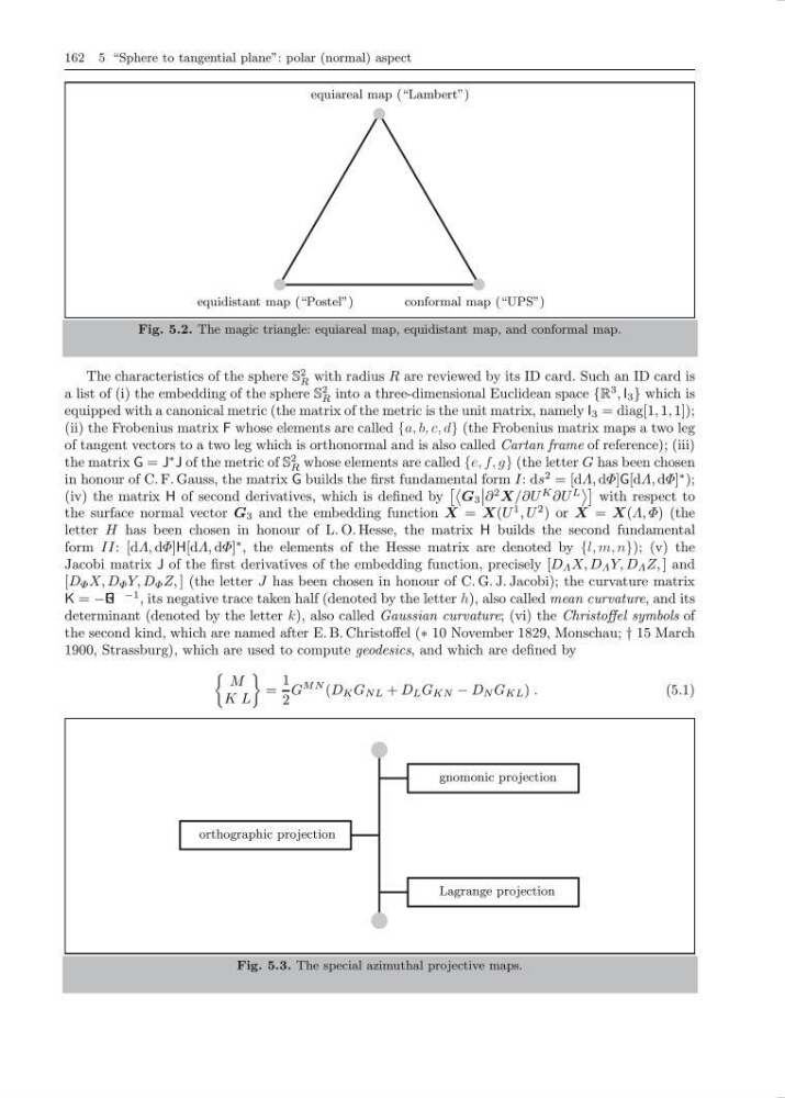
Fig. 5.2. The magic triangle: equiareal map, equidistant map, and conformal map.
The characteristics of the sphere S
2
R with radius R are reviewed by its ID card. Such an ID card is
a list of (i) the embedding of the sphere S
2
R into a three-dimensional Euclidean space {R
3 , I 3 } which is
equipped with a canonical metric (the matrix of the metric is the unit matrix, namely I 3 = diag[1, 1, 1]);
(ii) the Frobenius matrix F whose elements are called {a, b, c, d} (the Frobenius matrix maps a two leg
of tangent vectors to a two leg which is orthonormal and is also called Cartan frame of reference); (iii)
the matrix G = J
∗ J of the metric of S
2
R whose elements are called {e, f, g} (the letter G has been chosen
in honour of C. F. Gauss, the matrix G builds the first fundamental form I: ds
2 = [dΛ, dΦ]G[dΛ, dΦ]
∗ );
(iv) the matrix H of second derivatives, which is defined by
G 3
∂
2 X/∂U
K ∂U
L
with respect to
the surface normal vector G 3 and the embedding function X = X(U
1 , U
2 ) or X = X(Λ, Φ) (the
letter H has been chosen in honour of L. O. Hesse, the matrix H builds the second fundamental
form II: [dΛ, dΦ]H[dΛ, dΦ]
∗ , the elements of the Hesse matrix are denoted by {l, m, n}); (v) the
Jacobi matrix J of the first derivatives of the embedding function, precisely [D Λ X, D Λ Y, D Λ Z, ] and
[D Φ X, D Φ Y, D Φ Z, ] (the letter J has been chosen in honour of C. G. J. Jacobi); the curvature matrix
K = −H G
−1 , its negative trace taken half (denoted by the letter h), also called mean curvature, and its
determinant (denoted by the letter k), also called Gaussian curvature; (vi) the Christoffel symbols of
the second kind, which are named after E. B. Christoffel (∗ 10 November 1829, Monschau; † 15 March
1900, Strassburg), which are used to compute geodesics, and which are defined by
M
K L
=
1
2
G
MN (D K G NL + D L G KN − D N G KL ) .
(5.1)
gnomonic projection
orthographic projection
Lagrange projection
Fig. 5.3. The special azimuthal projective maps.
equiareal map (“Lambert”)
equidistant map (“Postel”)
conformal map (“UPS”)
Fig. 5.2. The magic triangle: equiareal map, equidistant map, and conformal map.
The characteristics of the sphere S
2
R with radius R are reviewed by its ID card. Such an ID card is
a list of (i) the embedding of the sphere S
2
R into a three-dimensional Euclidean space {R
3 , I 3 } which is
equipped with a canonical metric (the matrix of the metric is the unit matrix, namely I 3 = diag[1, 1, 1]);
(ii) the Frobenius matrix F whose elements are called {a, b, c, d} (the Frobenius matrix maps a two leg
of tangent vectors to a two leg which is orthonormal and is also called Cartan frame of reference); (iii)
the matrix G = J
∗ J of the metric of S
2
R whose elements are called {e, f, g} (the letter G has been chosen
in honour of C. F. Gauss, the matrix G builds the first fundamental form I: ds
2 = [dΛ, dΦ]G[dΛ, dΦ]
∗ );
(iv) the matrix H of second derivatives, which is defined by
G 3
∂
2 X/∂U
K ∂U
L
with respect to
the surface normal vector G 3 and the embedding function X = X(U
1 , U
2 ) or X = X(Λ, Φ) (the
letter H has been chosen in honour of L. O. Hesse, the matrix H builds the second fundamental
form II: [dΛ, dΦ]H[dΛ, dΦ]
∗ , the elements of the Hesse matrix are denoted by {l, m, n}); (v) the
Jacobi matrix J of the first derivatives of the embedding function, precisely [D Λ X, D Λ Y, D Λ Z, ] and
[D Φ X, D Φ Y, D Φ Z, ] (the letter J has been chosen in honour of C. G. J. Jacobi); the curvature matrix
K = −H G
−1 , its negative trace taken half (denoted by the letter h), also called mean curvature, and its
determinant (denoted by the letter k), also called Gaussian curvature; (vi) the Christoffel symbols of
the second kind, which are named after E. B. Christoffel (∗ 10 November 1829, Monschau; † 15 March
1900, Strassburg), which are used to compute geodesics, and which are defined by
M
K L
=
1
2
G
MN (D K G NL + D L G KN − D N G KL ) .
(5.1)
gnomonic projection
orthographic projection
Lagrange projection
Fig. 5.3. The special azimuthal projective maps.