

3-3 The oblique frame of reference of the sphere 139
Note that the direct transformation {λ, φ; λ
0 , φ 0 } → {α E , β} can then be conveniently solved, namely
with the result that is presented in Box 3.6. First, for the choice φ 0 = 0, sin(λ − λ 0 ) = cos(λ − λ
0 ),
cos(λ − λ 0 ) = − sin(λ − λ
0 ), and tan α = tan α S = −1/ tan α E = − cot α E , we have derived the
transverse equations of reference. Second, if we substitute these identities into the representative
formulae “from the equatorial frame of reference
e 1 , e 2 , e 3
O
to the meta-equatorial (“oblique”)
frame of reference
e 1 0 , e 2 0 , e 3 0
O
” that are collected in Box 3.5, we are directly led to the basic
identities of transforming from the equatorial reference frame to the transverse reference frame.
3-35 Transformations between oblique frames of reference: first design, second design
Question.
Question: “How can the two oblique frames of reference e
0 and E
, called first design and
second design, respectively, be related?” Answer: “The two oblique frames of reference can
be related to each other when we allow a third rotation in the Kepler orbital plane by means
of [E 1 , E 2 , E 3 ]
∗ = R 3 (ω)[E 1 , E 2 , E 3 ]
∗ .”
Note that ω is called longitude in the meta-equatorial plane. Such an additional rotation may come as a
surprise, but without such a longitude, the oblique frames of first and second kind cannot be identified
without inconsistencies. Sometimes, the angular parameter ω is called ambiguity. As it is outlined in
Box 3.18 and Box 3.19, the identity postulate (3.90) leads to trigonometric equations for {ω, I, Ω}
(given λ 0 and φ 0 ) and {λ 0 , φ 0 } (given ω, I, and Ω). Accordingly, we are able to transform forward
and backward between the oblique frames of reference subject to [E 1 , E 2 , E 3 ]
∗ = [e 1 0 , e 2 0 , e 3 0 ]
∗ ,
[E 1 , E 2 , E 3 ]
∗ = [e 1 , e 2 , e 3 ]
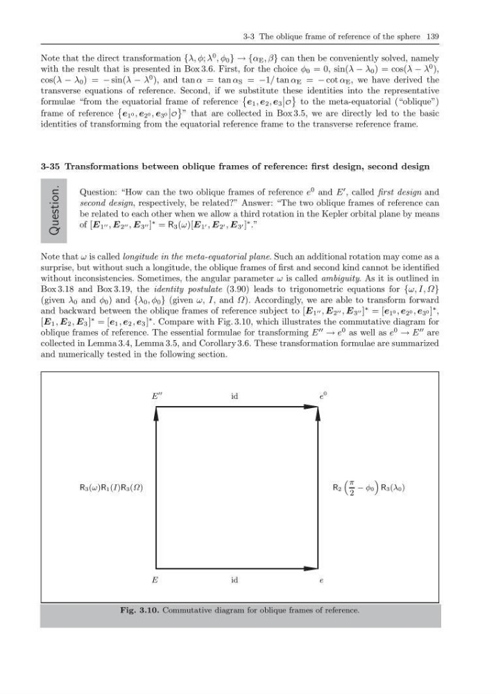
∗ . Compare with Fig. 3.10, which illustrates the commutative diagram for
oblique frames of reference. The essential formulae for transforming E
→ e
0 as well as e
0
→ E
are
collected in Lemma 3.4, Lemma 3.5, and Corollary 3.6. These transformation formulae are summarized
and numerically tested in the following section.
E
e
0
E
e
id
id
R3(ω)R 1 (I)R 3 (Ω)
R2
“ π
2
− φ 0
”
R3(λ 0 )
Fig. 3.10. Commutative diagram for oblique frames of reference.
Note that the direct transformation {λ, φ; λ
0 , φ 0 } → {α E , β} can then be conveniently solved, namely
with the result that is presented in Box 3.6. First, for the choice φ 0 = 0, sin(λ − λ 0 ) = cos(λ − λ
0 ),
cos(λ − λ 0 ) = − sin(λ − λ
0 ), and tan α = tan α S = −1/ tan α E = − cot α E , we have derived the
transverse equations of reference. Second, if we substitute these identities into the representative
formulae “from the equatorial frame of reference
e 1 , e 2 , e 3
O
to the meta-equatorial (“oblique”)
frame of reference
e 1 0 , e 2 0 , e 3 0
O
” that are collected in Box 3.5, we are directly led to the basic
identities of transforming from the equatorial reference frame to the transverse reference frame.
3-35 Transformations between oblique frames of reference: first design, second design
Question.
Question: “How can the two oblique frames of reference e
0 and E
, called first design and
second design, respectively, be related?” Answer: “The two oblique frames of reference can
be related to each other when we allow a third rotation in the Kepler orbital plane by means
of [E 1 , E 2 , E 3 ]
∗ = R 3 (ω)[E 1 , E 2 , E 3 ]
∗ .”
Note that ω is called longitude in the meta-equatorial plane. Such an additional rotation may come as a
surprise, but without such a longitude, the oblique frames of first and second kind cannot be identified
without inconsistencies. Sometimes, the angular parameter ω is called ambiguity. As it is outlined in
Box 3.18 and Box 3.19, the identity postulate (3.90) leads to trigonometric equations for {ω, I, Ω}
(given λ 0 and φ 0 ) and {λ 0 , φ 0 } (given ω, I, and Ω). Accordingly, we are able to transform forward
and backward between the oblique frames of reference subject to [E 1 , E 2 , E 3 ]
∗ = [e 1 0 , e 2 0 , e 3 0 ]
∗ ,
[E 1 , E 2 , E 3 ]
∗ = [e 1 , e 2 , e 3 ]
∗ . Compare with Fig. 3.10, which illustrates the commutative diagram for
oblique frames of reference. The essential formulae for transforming E
→ e
0 as well as e
0
→ E
are
collected in Lemma 3.4, Lemma 3.5, and Corollary 3.6. These transformation formulae are summarized
and numerically tested in the following section.
E
e
0
E
e
id
id
R3(ω)R 1 (I)R 3 (Ω)
R2
“ π
2
− φ 0
”
R3(λ 0 )
Fig. 3.10. Commutative diagram for oblique frames of reference.