2-4 The equivalence theorem for equiareal mappings 109
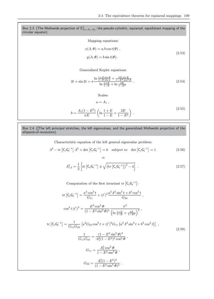
Box 2.3 (The Mollweide projection of E
2
A 1 ,A 1 ,A 2 ; the pseudo-cylindric, equiareal, equidistant mapping of the
circular equator).
Mapping equations:
x(Λ, Φ) = aΛ cos t(Φ) ,
y(Λ, Φ) = b sin t(Φ) .
(2.53)
Generalized Kepler equations:
2t + sin 2t = π
ln
1+E sin Φ
1−E sin φ
+
2E sin Φ
1−E 2 sin 2 Φ
ln
1+E
1−E
+ ln
2E
1−E 2
.
(2.54)
Scales:
a = A 1 ,
b =
A 1 (1 − E
2 )
πE
„
ln
1 + E
1 − E
+
2E
1 − E 2
«
.
(2.55)
Box 2.4 ([The left principal stretches, the left eigenvalues, and the generalized Mollweide projection of the
ellipsoid-of-revolution).
Characteristic equation of the left general eigenvalue problem:
Λ
4 − tr
ˆ
C l G
−1
l
˜
Λ
2 + det
ˆ
C l G
−1
l
˜
= 0 subject to det
ˆ
C l G
−1
l
˜
= 1
(2.56)
⇒
Λ
2
1,2 =
1
2
»
tr
ˆ
C l G
−1
l
˜ ±
q `
tr
ˆ
C l G
−1
l
˜´ 2 − 4
–
.
(2.57)
Computation of the first invariant tr
ˆ
C l G
−1
l
˜
:
tr
ˆ
C l G
−1
l
˜
=
a
2 cos
2 t
G 11
+ (t
)
2 a
2 Λ
2 sin
2 t + b
2 cos
2 t
G 22
,
cos
4 t (t
)
2 =
E
2 cos
2 Φ
(1 − E 2 sin
2 Φ) 4
π
2
“
ln
1+E
1−E
+
2E
1−E 2
” 2 ,
tr
ˆ
C l G
−1
l
˜
=
1
G 11 G 22
ˆ
a
2 G 22 cos
2 t + (t
)
2 G 11
`
a
2 Λ
2 sin
2 t + b
2 cos
2 t
´˜
,
1
G 11 G 22
=
(1 − E
2 sin
2 Φ)
4
A
4
1 (1 − E 2 ) 2 cos 2 Φ
,
G 11 =
A
2
1 cos
2 Φ
1 − E 2 sin
2 Φ
,
G 22 =
A
2
1 (1 − E
2 )
2
(1 − E 2 sin
2 Φ) 3 .
(2.58)