

2-3 The equivalence theorem for conformal mappings 103
Box 2.1 (Conformal diffeomorphism M
2
l → M
2
r = {R
2 , δ µν } = E
2 , exterior calculus).
Diffeomorphism:
»
dx
dy
–
= J l
»
dU
dV
–
or
»
dU
dV
–
= J r
»
dx
dy
–
⇔
J l = J
−1
r
⇔
J r = J
−1
l
.
(2.28)
Right Cauchy–Green matrix for a conformal diffeomorphism:
C r = J
T
r G l J r = λ
2 I 2
⇔
C
−1
r
= J l G
−1
l J
T
l = λ
−2 I 2 .
(2.29)
The rows of the left Jacobi matrix are G
−1
l
orthogonal:
dx = x U dU + x V dV =
2
X
M=1
x M dU
M , x 1 := D U x = x U , x 2 := D V x = x V .
(2.30)
Hodge star operator:
∗dy :=
2
X
L,M,N =1
e LM
p
det [G l ]G
MN y N dU
L ,
subject to
y 1 := D U y = y U , y 2 := D V y = y V .
(2.31)
Permutation symbol:
e LM =
8
<
:
+1 for an even permutation of the indices L, M ∈ {1, 2}
−1 for an odd permutation of the indices L, M ∈ {1, 2}
0
otherwise
.
(2.32)
Korn–Lichtenstein equations in exterior calculus:
dx =
2
X
M=1
x M dU
M =
2
X
L,M,N =1
e LM
p
det [G l ]G
MN y N dU
L = dy
∗
⇔
∂x
∂U L = e LM
p
det [G l ]G
MN ∂y
∂U N , dx = dy
∗ .
(2.33)
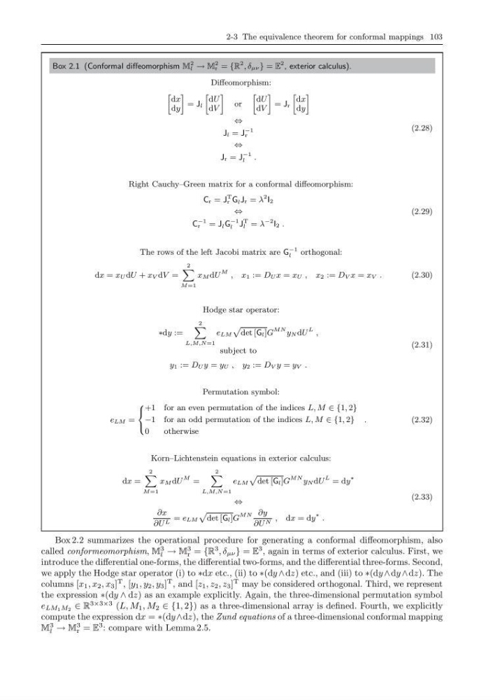
Box 2.2 summarizes the operational procedure for generating a conformal diffeomorphism, also
called conformeomorphism, M
3
l → M
3
r = {R
3 , δ µν } = E
3 , again in terms of exterior calculus. First, we
introduce the differential one-forms, the differential two-forms, and the differential three-forms. Second,
we apply the Hodge star operator (i) to ∗dx etc., (ii) to ∗(dy ∧ dz) etc., and (iii) to ∗(dy ∧ dy ∧ dz). The
columns [x 1 , x 2 , x 3 ]
T , [y 1 , y 2 , y 3 ]
T , and [z 1 , z 2 , z 3 ]
T may be considered orthogonal. Third, we represent
the expression ∗(dy ∧ dz) as an example explicitly. Again, the three-dimensional permutation symbol
e LM 1 M 2 ∈ R
3×3×3 (L, M 1 , M 2 ∈ {1, 2}) as a three-dimensional array is defined. Fourth, we explicitly
compute the expression dx = ∗(dy∧dz), the Zund equations of a three-dimensional conformal mapping
M
3
l → M
3
r = E
3 : compare with Lemma 2.5.
Box 2.1 (Conformal diffeomorphism M
2
l → M
2
r = {R
2 , δ µν } = E
2 , exterior calculus).
Diffeomorphism:
»
dx
dy
–
= J l
»
dU
dV
–
or
»
dU
dV
–
= J r
»
dx
dy
–
⇔
J l = J
−1
r
⇔
J r = J
−1
l
.
(2.28)
Right Cauchy–Green matrix for a conformal diffeomorphism:
C r = J
T
r G l J r = λ
2 I 2
⇔
C
−1
r
= J l G
−1
l J
T
l = λ
−2 I 2 .
(2.29)
The rows of the left Jacobi matrix are G
−1
l
orthogonal:
dx = x U dU + x V dV =
2
X
M=1
x M dU
M , x 1 := D U x = x U , x 2 := D V x = x V .
(2.30)
Hodge star operator:
∗dy :=
2
X
L,M,N =1
e LM
p
det [G l ]G
MN y N dU
L ,
subject to
y 1 := D U y = y U , y 2 := D V y = y V .
(2.31)
Permutation symbol:
e LM =
8
<
:
+1 for an even permutation of the indices L, M ∈ {1, 2}
−1 for an odd permutation of the indices L, M ∈ {1, 2}
0
otherwise
.
(2.32)
Korn–Lichtenstein equations in exterior calculus:
dx =
2
X
M=1
x M dU
M =
2
X
L,M,N =1
e LM
p
det [G l ]G
MN y N dU
L = dy
∗
⇔
∂x
∂U L = e LM
p
det [G l ]G
MN ∂y
∂U N , dx = dy
∗ .
(2.33)
Box 2.2 summarizes the operational procedure for generating a conformal diffeomorphism, also
called conformeomorphism, M
3
l → M
3
r = {R
3 , δ µν } = E
3 , again in terms of exterior calculus. First, we
introduce the differential one-forms, the differential two-forms, and the differential three-forms. Second,
we apply the Hodge star operator (i) to ∗dx etc., (ii) to ∗(dy ∧ dz) etc., and (iii) to ∗(dy ∧ dy ∧ dz). The
columns [x 1 , x 2 , x 3 ]
T , [y 1 , y 2 , y 3 ]
T , and [z 1 , z 2 , z 3 ]
T may be considered orthogonal. Third, we represent
the expression ∗(dy ∧ dz) as an example explicitly. Again, the three-dimensional permutation symbol
e LM 1 M 2 ∈ R
3×3×3 (L, M 1 , M 2 ∈ {1, 2}) as a three-dimensional array is defined. Fourth, we explicitly
compute the expression dx = ∗(dy∧dz), the Zund equations of a three-dimensional conformal mapping
M
3
l → M
3
r = E
3 : compare with Lemma 2.5.