

48
2. Hydrodynamic Dispersion in Porous Media
Let the radioaetive deeay eoefficient be A. and the retardation faetor be R d •
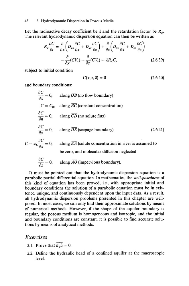
The relevant hydrodynamie dispersion equation ean then be written as
oC
0 (OC
OC) 0 (OC
OC)
Rrat = OX D xx OX + D xz OZ + OZ Dzx OX + D zz OZ
o
0
- ox (Cy") - oz (C~) - A.RdC,
(2.6.39)
subjeet to initial eondition
C(X,Z,O) = °
and boundary eonditions:
~~ = 0, along OB (no flow boundary)
C = Co, along BC (eonstant eoneentration)
~~ = 0, along CD (no solute flux)
oC =0
ox '
along DE (seepage boundary)
(2.6.40)
(2.6.41)
oC
C - (XL OX = 0,
along EA (solute eoneentration in river is assumed to
be zero, and moleeular diffusion negleeted
~~ = 0, along AO (impervious boundary).
It must be pointed out that the hydrodynamie dispersion equation is a
parabolie partial differential equation. In mathematies, the well-posedness of
this kind of equation has been proved, i.e., with appropriate initial and
boundary eonditions the solution of a parabolie equation must be in existenee, unique, and eontinuously dependent upon the input data. As a result,
all hydrodynamie dispersion problems presented in this ehapter are wellposed. In most eases, we ean only find their approximate solutions by means
of numerieal methods. However, if the shape of the aquifer boundary is
regular, the porous medium is homogeneous and isotropie, and the initial
and boundary eonditions are eonstant, it is possible to find aeeurate solutions by means of analytieal methods.
Exercises
2.1. Prove that ä 1 ä = 0.
2.2. Define the hydraulic head of a eonfined aquifer at the maeroseopie
level.
2. Hydrodynamic Dispersion in Porous Media
Let the radioaetive deeay eoefficient be A. and the retardation faetor be R d •
The relevant hydrodynamie dispersion equation ean then be written as
oC
0 (OC
OC) 0 (OC
OC)
Rrat = OX D xx OX + D xz OZ + OZ Dzx OX + D zz OZ
o
0
- ox (Cy") - oz (C~) - A.RdC,
(2.6.39)
subjeet to initial eondition
C(X,Z,O) = °
and boundary eonditions:
~~ = 0, along OB (no flow boundary)
C = Co, along BC (eonstant eoneentration)
~~ = 0, along CD (no solute flux)
oC =0
ox '
along DE (seepage boundary)
(2.6.40)
(2.6.41)
oC
C - (XL OX = 0,
along EA (solute eoneentration in river is assumed to
be zero, and moleeular diffusion negleeted
~~ = 0, along AO (impervious boundary).
It must be pointed out that the hydrodynamie dispersion equation is a
parabolie partial differential equation. In mathematies, the well-posedness of
this kind of equation has been proved, i.e., with appropriate initial and
boundary eonditions the solution of a parabolie equation must be in existenee, unique, and eontinuously dependent upon the input data. As a result,
all hydrodynamie dispersion problems presented in this ehapter are wellposed. In most eases, we ean only find their approximate solutions by means
of numerieal methods. However, if the shape of the aquifer boundary is
regular, the porous medium is homogeneous and isotropie, and the initial
and boundary eonditions are eonstant, it is possible to find aeeurate solutions by means of analytieal methods.
Exercises
2.1. Prove that ä 1 ä = 0.
2.2. Define the hydraulic head of a eonfined aquifer at the maeroseopie
level.