

46
2. Hydrodynamic Dispersion in Porous Media
A
iJe =0
()y
B
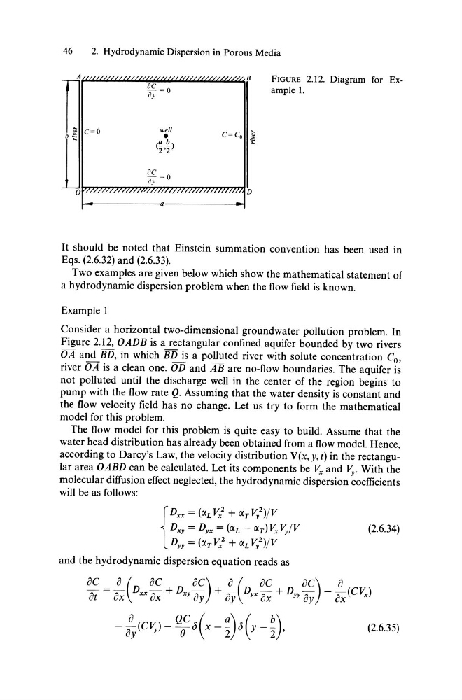
FIGURE 2.12. Diagram for Example 1.
t c=o
b .~
c=co .~
~-----------a----------~~
It should be noted that Einstein summation convention has been used in
Eqs. (2.6.32) and (2.6.33).
Two ex am pies are given below wh ich show the mathematical statement of
a hydrodynamic dispersion problem when the flow field is known.
Example 1
Consider a horizontal two-dimensional groundwater pollution problem. In
Figure 2.12, OADB is a rectangular confined aquifer bounded by two rivers
OA and BD, in which BD is apolluted river with solute concentration Co,
river OA is a clean one. OD and AB are no-flow boundaries. The aquifer is
not polluted until the discharge weIl in the center of the region begins to
pump with the flow rate Q. Assuming that the water density is constant and
the flow velocity field has no change. Let us try to form the mathematical
model for this problem.
The flow model for this problem is quite easy to build. Assume that the
water head distribution has already been obtained from a flow model. Hence,
according to Darcy's Law, the velocity distribution V(x,y, t) in the rectangular area OABD can be ca1culated. Let its components be V x and Vy. With the
molecular diffusion effect neglected, the hydrodynamic dispersion coefficients
will be as follows:
{
DXX = (CXL Vx 2 + CX T Vy2)jV
Dxy = Dyx = (cxL - cxT)Vx VyjV
Dyy = (CXT V/ + CXL ~,2)jV
and the hydrodynamic dispersion equation reads as
(2.6.34)
(2.6.35)
2. Hydrodynamic Dispersion in Porous Media
A
iJe =0
()y
B
FIGURE 2.12. Diagram for Example 1.
t c=o
b .~
c=co .~
~-----------a----------~~
It should be noted that Einstein summation convention has been used in
Eqs. (2.6.32) and (2.6.33).
Two ex am pies are given below wh ich show the mathematical statement of
a hydrodynamic dispersion problem when the flow field is known.
Example 1
Consider a horizontal two-dimensional groundwater pollution problem. In
Figure 2.12, OADB is a rectangular confined aquifer bounded by two rivers
OA and BD, in which BD is apolluted river with solute concentration Co,
river OA is a clean one. OD and AB are no-flow boundaries. The aquifer is
not polluted until the discharge weIl in the center of the region begins to
pump with the flow rate Q. Assuming that the water density is constant and
the flow velocity field has no change. Let us try to form the mathematical
model for this problem.
The flow model for this problem is quite easy to build. Assume that the
water head distribution has already been obtained from a flow model. Hence,
according to Darcy's Law, the velocity distribution V(x,y, t) in the rectangular area OABD can be ca1culated. Let its components be V x and Vy. With the
molecular diffusion effect neglected, the hydrodynamic dispersion coefficients
will be as follows:
{
DXX = (CXL Vx 2 + CX T Vy2)jV
Dxy = Dyx = (cxL - cxT)Vx VyjV
Dyy = (CXT V/ + CXL ~,2)jV
and the hydrodynamic dispersion equation reads as
(2.6.34)
(2.6.35)