

1.2. Groundwater Quality Management
3
serious consequences, such as the depletion of water, the deterioration of
water quality, and the subsidence of land.
When the groundwater system is utilized in accordance with some special
purposes and demands, it is necessary to make some decisions. For example,
if the aquifer is regarded as a supply source, then the location, yield, the
number of the pumping weIls, as weIl as the water quantity and quality of
artificial recharge, must be determined. There are many ways to reach the
same objective, so the factors mentioned above should be regarded as variables, wh ich are caIled decision variables.
However, not aIl the decisions are feasible. The decision variables must
obey certain restrictions which are caIled constraints. Suppose that an aquifer
management plan is beneficial in one aspect, but causes the water table to
decline on a large scale. If either the pumping weIls are unable to draw water
Or poIluted water comes from a neighboring region, the plan is not feasible.
In mathematical terms, we say that the relevant decision variables do not
satisfy the restrictive conditions Or constraints.
In general cases, there are a number of feasible decisions which satisfy aIl
of the restricted conditions. Thus, an important problem is how to select the
optimal decision. Before solving this problem, we must set up so me criteria
for judging "bad" Or "good" decisions. For example, the cost ofwater per ton
may be taken as a criterion. Since different decisions correspond with different costs, the optimal decision can be selected as the one with the lowest cost.
The selected criteria, which are functions of decision variables, are called
objective functions. The minimum (or maximum) of an objective function is a
goal that we endeavor to achieve. The management of groundwater then
becomes the selection of the optimal feasible decision Or decisions for attaining one Or several goals. Mathematically, it involves solving the following
single- Or multiple-objective optimization problem with aseries of constraints:
minJ(q),
subject to
h(q; Xi' t) :2: !!i , (i = 1,2, ... , I),
C~(q; Xj' t) :5: C~.j' (j = 1,2, ... , J).
(1.2.1)
(1.2.2)
(1.2.3)
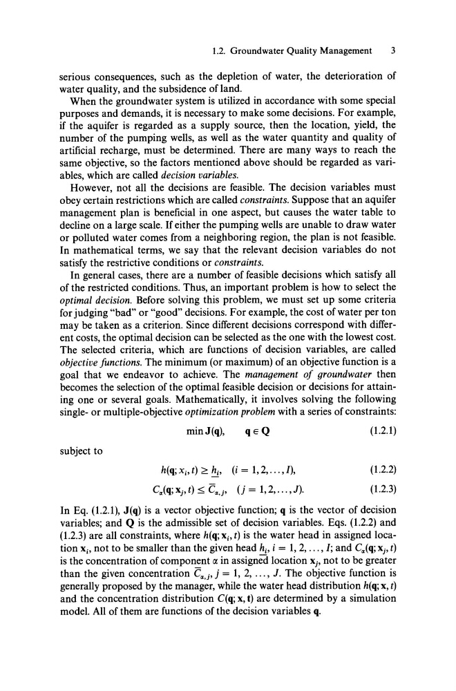
In Eq. (1.2.1), J(q) is a vectOr objective function; q is the vector of decision
variables; and Q is the admissible set of decision variables. Eqs. (1.2.2) and
(1.2.3) are all constraints, where h(q; Xi' t) is the water head in assigned locati on Xi' not to be sm aller than the given head hi , i = 1,2, ... , I; and C~(q; Xj' t)
is the concentration of component r:J. in assigned location Xj' not to be greater
than the given concentration C~.j' j = 1, 2, ... , J. The objective function is
generaIly proposed by the manager, while the water head distribution h(q; X, t)
and the concentration distribution C(q; X, t) are determined by a simulation
model. All of them are functions of the decision variables q.
3
serious consequences, such as the depletion of water, the deterioration of
water quality, and the subsidence of land.
When the groundwater system is utilized in accordance with some special
purposes and demands, it is necessary to make some decisions. For example,
if the aquifer is regarded as a supply source, then the location, yield, the
number of the pumping weIls, as weIl as the water quantity and quality of
artificial recharge, must be determined. There are many ways to reach the
same objective, so the factors mentioned above should be regarded as variables, wh ich are caIled decision variables.
However, not aIl the decisions are feasible. The decision variables must
obey certain restrictions which are caIled constraints. Suppose that an aquifer
management plan is beneficial in one aspect, but causes the water table to
decline on a large scale. If either the pumping weIls are unable to draw water
Or poIluted water comes from a neighboring region, the plan is not feasible.
In mathematical terms, we say that the relevant decision variables do not
satisfy the restrictive conditions Or constraints.
In general cases, there are a number of feasible decisions which satisfy aIl
of the restricted conditions. Thus, an important problem is how to select the
optimal decision. Before solving this problem, we must set up so me criteria
for judging "bad" Or "good" decisions. For example, the cost ofwater per ton
may be taken as a criterion. Since different decisions correspond with different costs, the optimal decision can be selected as the one with the lowest cost.
The selected criteria, which are functions of decision variables, are called
objective functions. The minimum (or maximum) of an objective function is a
goal that we endeavor to achieve. The management of groundwater then
becomes the selection of the optimal feasible decision Or decisions for attaining one Or several goals. Mathematically, it involves solving the following
single- Or multiple-objective optimization problem with aseries of constraints:
minJ(q),
subject to
h(q; Xi' t) :2: !!i , (i = 1,2, ... , I),
C~(q; Xj' t) :5: C~.j' (j = 1,2, ... , J).
(1.2.1)
(1.2.2)
(1.2.3)
In Eq. (1.2.1), J(q) is a vectOr objective function; q is the vector of decision
variables; and Q is the admissible set of decision variables. Eqs. (1.2.2) and
(1.2.3) are all constraints, where h(q; Xi' t) is the water head in assigned locati on Xi' not to be sm aller than the given head hi , i = 1,2, ... , I; and C~(q; Xj' t)
is the concentration of component r:J. in assigned location Xj' not to be greater
than the given concentration C~.j' j = 1, 2, ... , J. The objective function is
generaIly proposed by the manager, while the water head distribution h(q; X, t)
and the concentration distribution C(q; X, t) are determined by a simulation
model. All of them are functions of the decision variables q.