

5.2. The Multiple Cell Balance Method
117
tion of each point can be represented approximately by linear interpolation
of its nodal values, i.e.,
C(x, y, t) = (Mx, y)C;(t) +
where interpolation functions
1
(5.2.4)
(5.2.5)
are just the basis functions of linear FEM (see Eq. (5.1.32)). C;(t), Cj(t), Ck(t)
in Eq. (5.2.4) are the solute concentrations of nodes i, j, k at time t, respectively. Coefficients a" b" and c, in the above equation are given by Eq.
(5.1.33), ~e is the area of element (e).
From Eq. (5.2.4) we can directly obtain the following expressions for element (e):
OC
1
ox = 2~e (biC; + bjCj + bkCk),
(5.2.6)
oC
1
a = 2~ (CiCi + CjCj + CkCk),
Y
e
(5.2.7)
oC =
I ot
J ot
ot
(5.2.8)
Saturated thickness m, head hand velocity components V x , V, can also be
represented by the same linear interpolation functions defined in Eq. (5.2.5).
Now let us consider all the elements with node i as one of their vertices.
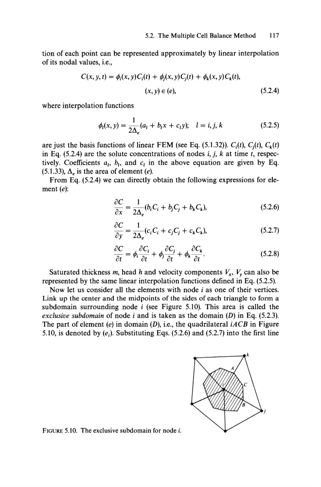
Link up the center and the midpoints of the sides of each triangle to form a
subdomain surrounding node i (see Figure 5.10). This area is called the
exclusive subdomain of node i and is taken as the domain (D) in Eq. (5.2.3).
The part of element (e) in domain (D), i.e., the quadrilateral iACB in Figure
5.10, is denoted by (e;). Substituting Eqs. (5.2.6) and (5.2.7) into the first line
FIGURE 5.10. The exclusive subdomain for node i.
117
tion of each point can be represented approximately by linear interpolation
of its nodal values, i.e.,
C(x, y, t) = (Mx, y)C;(t) +
where interpolation functions
1
(5.2.4)
(5.2.5)
are just the basis functions of linear FEM (see Eq. (5.1.32)). C;(t), Cj(t), Ck(t)
in Eq. (5.2.4) are the solute concentrations of nodes i, j, k at time t, respectively. Coefficients a" b" and c, in the above equation are given by Eq.
(5.1.33), ~e is the area of element (e).
From Eq. (5.2.4) we can directly obtain the following expressions for element (e):
OC
1
ox = 2~e (biC; + bjCj + bkCk),
(5.2.6)
oC
1
a = 2~ (CiCi + CjCj + CkCk),
Y
e
(5.2.7)
oC =
I ot
J ot
ot
(5.2.8)
Saturated thickness m, head hand velocity components V x , V, can also be
represented by the same linear interpolation functions defined in Eq. (5.2.5).
Now let us consider all the elements with node i as one of their vertices.
Link up the center and the midpoints of the sides of each triangle to form a
subdomain surrounding node i (see Figure 5.10). This area is called the
exclusive subdomain of node i and is taken as the domain (D) in Eq. (5.2.3).
The part of element (e) in domain (D), i.e., the quadrilateral iACB in Figure
5.10, is denoted by (e;). Substituting Eqs. (5.2.6) and (5.2.7) into the first line
FIGURE 5.10. The exclusive subdomain for node i.