

5.1. Finite Element Methods for Two-Dimensional Problems
105
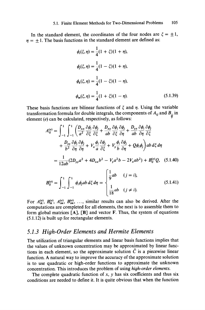
In the standard element, the coordinates of the four nodes are ~ = ± 1,
I] = ± 1. The basis functions in the standard element are defined as:
1
(M~,I]) = 4(1 + ~)(1 + 1]),
1
These basis functions are bilinear functions of ~ and 1]. Using the variable
transformation formula for double integrals, the components of Aij and B .. in
element (e) can be calculated, respectively, as follows:
1J
A\~) = f 1 f 1 (Dxx O
-1
-1
a 2 O~ o~
ab o~ 01]
ab 01] o~
+ D yy O
x a o~
y b 01]
'f'1'f')
a .. I]
= 1;ab (2Dyy a 2 + 4Dxx b 2 - Yya 2 b - 2Vx ab 2 ) + Bif)Q, (5.1.40)
j
!ab
(j = i),
Bif) = L1 L1
(5.1.41)
For Al~), BI:), Al:::, Bl:::, ... , similar results can also be derived. After the
computations are completed for all elements, the next is to assemble them to
form global matrices [A], [B] and vector F. Thus, the system of equations
(5.1.12) is built up for rectangular elements.
5.1.3 High-Order Elements and Hermite Elements
The utilization of triangular elements and linear basis functions implies that
the values of unknown concentration may be approximated by linear functions in each element, so the approximate solution C is a piecewise linear
function. A natural way to improve the accuracy of the approximate solution
is to use quadratic or high-order functions to approximate the unknown
concentration. This introduces the problem of using high-order elements.
The complete quadratic function of x, y has six coefficients and thus six
conditions are needed to define it. It is quite obvious that when the function
105
In the standard element, the coordinates of the four nodes are ~ = ± 1,
I] = ± 1. The basis functions in the standard element are defined as:
1
(M~,I]) = 4(1 + ~)(1 + 1]),
1
These basis functions are bilinear functions of ~ and 1]. Using the variable
transformation formula for double integrals, the components of Aij and B .. in
element (e) can be calculated, respectively, as follows:
1J
A\~) = f 1 f 1 (Dxx O
-1
-1
a 2 O~ o~
ab o~ 01]
ab 01] o~
+ D yy O
x a o~
y b 01]
'f'1'f')
a .. I]
= 1;ab (2Dyy a 2 + 4Dxx b 2 - Yya 2 b - 2Vx ab 2 ) + Bif)Q, (5.1.40)
j
!ab
(j = i),
Bif) = L1 L1
(5.1.41)
For Al~), BI:), Al:::, Bl:::, ... , similar results can also be derived. After the
computations are completed for all elements, the next is to assemble them to
form global matrices [A], [B] and vector F. Thus, the system of equations
(5.1.12) is built up for rectangular elements.
5.1.3 High-Order Elements and Hermite Elements
The utilization of triangular elements and linear basis functions implies that
the values of unknown concentration may be approximated by linear functions in each element, so the approximate solution C is a piecewise linear
function. A natural way to improve the accuracy of the approximate solution
is to use quadratic or high-order functions to approximate the unknown
concentration. This introduces the problem of using high-order elements.
The complete quadratic function of x, y has six coefficients and thus six
conditions are needed to define it. It is quite obvious that when the function