

90
4. Finite DifTerence Methods
no-flow
boundary
CI Co
FIGURE 4.9. Mirror image on a no-flow boundary. 0 = previous
location of the partic1e; x = new location of the partic1e; .. =
point of the mirror image.
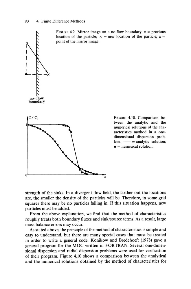
FIGURE 4.10. Comparison between the analytic and the
numerical solutions of the characteristics method in a onedimensional dispersion problem. - - = analytic solution;
• = numerical solution.
oL---------------~~~~x
strength of the sinks. In a divergent flow field, the farther out the locations
are, the sm aller the density of the particles will be. Therefore, in some grid
squares there may be no particles falling in. If this situation happens, new
particles must be added.
From the above explanation, we find that the method of characteristics
roughly treats both boundary fluxes and sink/source terms. As a result, large
mass balance errors may occur.
As stated above, the principle ofthe method of characteristics is simple and
easy to understand, but there are many special cases that must be treated
in order to write a general code. Konikow and Bredehoeft (1978) gave a
general program for the MOC written in FORTRAN. Several one-dimensional dispersion and radial dispersion problems were used for verification
of their program. Figure 4.10 shows a comparison between the analytical
and the numerical solutions obtained by the method of characteristics for
4. Finite DifTerence Methods
no-flow
boundary
CI Co
FIGURE 4.9. Mirror image on a no-flow boundary. 0 = previous
location of the partic1e; x = new location of the partic1e; .. =
point of the mirror image.
FIGURE 4.10. Comparison between the analytic and the
numerical solutions of the characteristics method in a onedimensional dispersion problem. - - = analytic solution;
• = numerical solution.
oL---------------~~~~x
strength of the sinks. In a divergent flow field, the farther out the locations
are, the sm aller the density of the particles will be. Therefore, in some grid
squares there may be no particles falling in. If this situation happens, new
particles must be added.
From the above explanation, we find that the method of characteristics
roughly treats both boundary fluxes and sink/source terms. As a result, large
mass balance errors may occur.
As stated above, the principle ofthe method of characteristics is simple and
easy to understand, but there are many special cases that must be treated
in order to write a general code. Konikow and Bredehoeft (1978) gave a
general program for the MOC written in FORTRAN. Several one-dimensional dispersion and radial dispersion problems were used for verification
of their program. Figure 4.10 shows a comparison between the analytical
and the numerical solutions obtained by the method of characteristics for