

50
D. Parra-Guevara and Y.N. Skiba
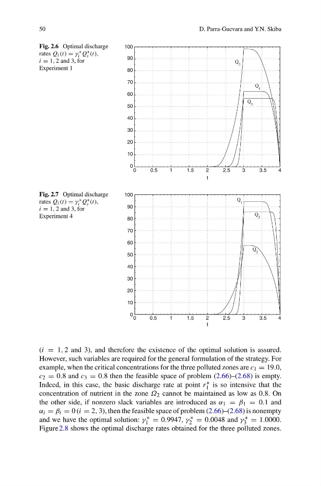
Fig. 2.6 Optimal discharge
rates Q i (t) = γ ∗
i Q ∗
i (t),
i = 1, 2 and 3, for
Experiment 1
0
0.5
1
1.5
2
2.5
3
3.5
4
0
10
20
30
40
50
60
70
80
90
100
t
Q
2
Q
1
Q 3
Fig. 2.7 Optimal discharge
rates Q i (t) = γ ∗
i Q ∗
i (t),
i = 1, 2 and 3, for
Experiment 4
0
0.5
1
1.5
2
2.5
3
3.5
4
0
10
20
30
40
50
60
70
80
90
100
t
Q
2
Q 1
Q
3
(i = 1, 2 and 3), and therefore the existence of the optimal solution is assured.
However, such variables are required for the general formulation of the strategy. For
example, when the critical concentrations for the three polluted zones are c 1 = 19.0,
c 2 = 0.8 and c 3 = 0.8 then the feasible space of problem (2.66)–(2.68) is empty.
Indeed, in this case, the basic discharge rate at point r ∗
1 is so intensive that the
concentration of nutrient in the zone Ω 2 cannot be maintained as low as 0.8. On
the other side, if nonzero slack variables are introduced as α 1 = β 1 = 0.1 and
α i = β i = 0 (i = 2, 3), then the feasible space of problem (2.66)–(2.68) is nonempty
and we have the optimal solution: γ ∗
1 = 0.9947, γ ∗
2 = 0.0048 and γ ∗
3 = 1.0000.
Figure 2.8 shows the optimal discharge rates obtained for the three polluted zones.
D. Parra-Guevara and Y.N. Skiba
Fig. 2.6 Optimal discharge
rates Q i (t) = γ ∗
i Q ∗
i (t),
i = 1, 2 and 3, for
Experiment 1
0
0.5
1
1.5
2
2.5
3
3.5
4
0
10
20
30
40
50
60
70
80
90
100
t
Q
2
Q
1
Q 3
Fig. 2.7 Optimal discharge
rates Q i (t) = γ ∗
i Q ∗
i (t),
i = 1, 2 and 3, for
Experiment 4
0
0.5
1
1.5
2
2.5
3
3.5
4
0
10
20
30
40
50
60
70
80
90
100
t
Q
2
Q 1
Q
3
(i = 1, 2 and 3), and therefore the existence of the optimal solution is assured.
However, such variables are required for the general formulation of the strategy. For
example, when the critical concentrations for the three polluted zones are c 1 = 19.0,
c 2 = 0.8 and c 3 = 0.8 then the feasible space of problem (2.66)–(2.68) is empty.
Indeed, in this case, the basic discharge rate at point r ∗
1 is so intensive that the
concentration of nutrient in the zone Ω 2 cannot be maintained as low as 0.8. On
the other side, if nonzero slack variables are introduced as α 1 = β 1 = 0.1 and
α i = β i = 0 (i = 2, 3), then the feasible space of problem (2.66)–(2.68) is nonempty
and we have the optimal solution: γ ∗
1 = 0.9947, γ ∗
2 = 0.0048 and γ ∗
3 = 1.0000.
Figure 2.8 shows the optimal discharge rates obtained for the three polluted zones.