

2 A Strategy for Bioremediation of Marine Shorelines …
47
2.7 Numerical Examples of Remediation in a Channel
In order to illustrate the method developed we now consider a two-dimensional example of remediation in a channel of one hundred and twenty metres long [0, 120] and
ten metres wide [0, 10]. The channel contains three oil-polluted zones Ω i (N = 3).
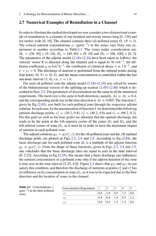
The critical nutrient concentrations c i (grm] −3 ) in the zones vary from one experiment to another according to Table 2.1. The zones under consideration are:
Ω 1 = [20, 30] × [9, 10], Ω 2 = [40, 60] × [9, 10] and Ω 3 = [96, 100] × [0, 2].
The parameters of the adjoint model (2.18)–(2.24) have been taken as follows: the
velocity vector U is directed along the channel and is equal to 30 m h −1 , the diffusion coefficient μ is 6 m 2 h −1 , the coefficient of chemical decay σ is 1 h −1 , and
ζ = v s = 0. The discharge of nutrient is performed from the optimal points during
four hours, (0, T ) ≡ (0, 4), and the mean concentration is controlled within the last
one-hour interval (3, 4), i.e., τ = 1 h.
For each oil polluted zone the adjoint model (2.18)–(2.24) was solved by means
of the bidimensional version of the splitting-up method (2.45)–(2.46) which is described in Sect. 2.5. The parameters of discretization are the same in all the numerical
experiments. The mesh size is the same in both directions, namely, Δx = Δy = 0.4,
and the corresponding mesh size in the time direction is Δt = 0.005. The function I ,
given by Eq. (2.63), was built for each polluted zone through the respective adjoint
solution. In each case, by the maximization of function I we determined the following
optimal discharge points: r ∗
1 = (20.2, 9.8), r ∗
2 = (40.2, 9.8) and r ∗
3 = (96.2, 0.2).
For this grid (as well as for finer grids) we obtained that the optimal discharge site
tends to be the point at the left-superior corner of the zones Ω 1 and Ω 2 , and the
left-inferior corner of zone Ω 3 , as it must be in order to have the maximum impact
of nutrient in each polluted zone.
The adjoint solutions g i j = g i (r ∗
j , t), for the ith polluted zone and the jth optimal
discharge point, are plotted in Figs. 2.3, 2.4 and 2.5. According to Eq. (2.64), the
basic discharge rate for each polluted zone Ω i is a multiple of the adjoint function
g ii = g i (r ∗
i , t). From the shape of these functions, given in Figs. 2.3, 2.4 and 2.5,
one concludes that the basic discharge rates are equal to zero in the time interval
[0, 2.25]. According to Eq. (2.25), this means that a basic discharge rate influences
the nutrient concentration of a polluted zone only if the adjoint function of the zone
is non-zero in the time interval [2.25, 4.0]. Figure 2.3 shows that g 12 and g 13 do not
satisfy this condition, and therefore the discharge of nutrients at points r ∗
2 and r ∗
3 has
no influence on its concentration in zone Ω 1 , as it was to be expected due to the flow
direction and the location of zones in the channel.
Table 2.1 Concentrations c i
(grm −3 ) in the three polluted
zones
Concentration\Experiment 1
2
3
4
5
c 1
0.8 1.0 0.5 1.2 0.6
c 2
0.8 0.8 1.0 0.5 1.2
c 3
0.8 0.5 1.5 1.2 0.6
47
2.7 Numerical Examples of Remediation in a Channel
In order to illustrate the method developed we now consider a two-dimensional example of remediation in a channel of one hundred and twenty metres long [0, 120] and
ten metres wide [0, 10]. The channel contains three oil-polluted zones Ω i (N = 3).
The critical nutrient concentrations c i (grm] −3 ) in the zones vary from one experiment to another according to Table 2.1. The zones under consideration are:
Ω 1 = [20, 30] × [9, 10], Ω 2 = [40, 60] × [9, 10] and Ω 3 = [96, 100] × [0, 2].
The parameters of the adjoint model (2.18)–(2.24) have been taken as follows: the
velocity vector U is directed along the channel and is equal to 30 m h −1 , the diffusion coefficient μ is 6 m 2 h −1 , the coefficient of chemical decay σ is 1 h −1 , and
ζ = v s = 0. The discharge of nutrient is performed from the optimal points during
four hours, (0, T ) ≡ (0, 4), and the mean concentration is controlled within the last
one-hour interval (3, 4), i.e., τ = 1 h.
For each oil polluted zone the adjoint model (2.18)–(2.24) was solved by means
of the bidimensional version of the splitting-up method (2.45)–(2.46) which is described in Sect. 2.5. The parameters of discretization are the same in all the numerical
experiments. The mesh size is the same in both directions, namely, Δx = Δy = 0.4,
and the corresponding mesh size in the time direction is Δt = 0.005. The function I ,
given by Eq. (2.63), was built for each polluted zone through the respective adjoint
solution. In each case, by the maximization of function I we determined the following
optimal discharge points: r ∗
1 = (20.2, 9.8), r ∗
2 = (40.2, 9.8) and r ∗
3 = (96.2, 0.2).
For this grid (as well as for finer grids) we obtained that the optimal discharge site
tends to be the point at the left-superior corner of the zones Ω 1 and Ω 2 , and the
left-inferior corner of zone Ω 3 , as it must be in order to have the maximum impact
of nutrient in each polluted zone.
The adjoint solutions g i j = g i (r ∗
j , t), for the ith polluted zone and the jth optimal
discharge point, are plotted in Figs. 2.3, 2.4 and 2.5. According to Eq. (2.64), the
basic discharge rate for each polluted zone Ω i is a multiple of the adjoint function
g ii = g i (r ∗
i , t). From the shape of these functions, given in Figs. 2.3, 2.4 and 2.5,
one concludes that the basic discharge rates are equal to zero in the time interval
[0, 2.25]. According to Eq. (2.25), this means that a basic discharge rate influences
the nutrient concentration of a polluted zone only if the adjoint function of the zone
is non-zero in the time interval [2.25, 4.0]. Figure 2.3 shows that g 12 and g 13 do not
satisfy this condition, and therefore the discharge of nutrients at points r ∗
2 and r ∗
3 has
no influence on its concentration in zone Ω 1 , as it was to be expected due to the flow
direction and the location of zones in the channel.
Table 2.1 Concentrations c i
(grm −3 ) in the three polluted
zones
Concentration\Experiment 1
2
3
4
5
c 1
0.8 1.0 0.5 1.2 0.6
c 2
0.8 0.8 1.0 0.5 1.2
c 3
0.8 0.5 1.5 1.2 0.6