

2 A Strategy for Bioremediation of Marine Shorelines …
27
in the oil-contaminated areas due to the slow degradation of the oil in the marine
environment. Sufficient conditions for such a methodology are given in Sect. 2.3.
2.2 Dispersion Model
The concentration of nutrient φ(r, t) in a bounded domain D ⊂ R 3 and time interval
[0, T ] is estimated by the following dispersion model
∂φ
∂t
+ U · ∇φ − ∇ · μ∇φ + σ φ + ∇ · φ s =
N
i=1
Q i (t)δ(r − r i )
(2.4)
φ s = −v s φk , in D
(2.5)
μ
∂φ
∂n
= φ s · n − ζ φk · n on S T
(2.6)
μ
∂φ
∂n
= 0 on S
+
(2.7)
μ
∂φ
∂n
− U n φ = 0 on S
−
(2.8)
μ
∂φ
∂n
= 0 on S B
(2.9)
φ(r, 0) = φ
0
(r ) in D
(2.10)
∇ · U = 0 in D.
(2.11)
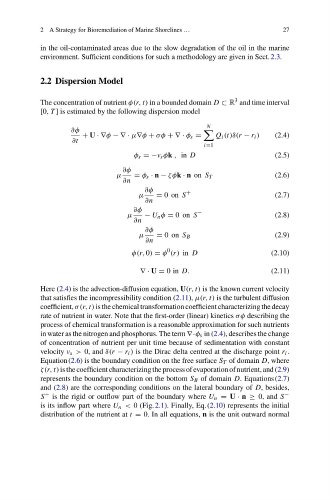
Here (2.4) is the advection-diffusion equation, U(r, t) is the known current velocity
that satisfies the incompressibility condition (2.11), μ(r, t) is the turbulent diffusion
coefficient, σ (r, t) is the chemical transformation coefficient characterizing the decay
rate of nutrient in water. Note that the first-order (linear) kinetics σ φ describing the
process of chemical transformation is a reasonable approximation for such nutrients
in water as the nitrogen and phosphorus. The term ∇ ·φ s in (2.4), describes the change
of concentration of nutrient per unit time because of sedimentation with constant
velocity v s > 0, and δ(r − r i ) is the Dirac delta centred at the discharge point r i .
Equation (2.6) is the boundary condition on the free surface S T of domain D, where
ζ(r, t) is the coefficient characterizing the process of evaporation of nutrient, and (2.9)
represents the boundary condition on the bottom S B of domain D. Equations (2.7)
and (2.8) are the corresponding conditions on the lateral boundary of D, besides,
S + is the rigid or outflow part of the boundary where U n = U · n ≥ 0, and S −
is its inflow part where U n < 0 (Fig. 2.1). Finally, Eq. (2.10) represents the initial
distribution of the nutrient at t = 0. In all equations, n is the unit outward normal
27
in the oil-contaminated areas due to the slow degradation of the oil in the marine
environment. Sufficient conditions for such a methodology are given in Sect. 2.3.
2.2 Dispersion Model
The concentration of nutrient φ(r, t) in a bounded domain D ⊂ R 3 and time interval
[0, T ] is estimated by the following dispersion model
∂φ
∂t
+ U · ∇φ − ∇ · μ∇φ + σ φ + ∇ · φ s =
N
i=1
Q i (t)δ(r − r i )
(2.4)
φ s = −v s φk , in D
(2.5)
μ
∂φ
∂n
= φ s · n − ζ φk · n on S T
(2.6)
μ
∂φ
∂n
= 0 on S
+
(2.7)
μ
∂φ
∂n
− U n φ = 0 on S
−
(2.8)
μ
∂φ
∂n
= 0 on S B
(2.9)
φ(r, 0) = φ
0
(r ) in D
(2.10)
∇ · U = 0 in D.
(2.11)
Here (2.4) is the advection-diffusion equation, U(r, t) is the known current velocity
that satisfies the incompressibility condition (2.11), μ(r, t) is the turbulent diffusion
coefficient, σ (r, t) is the chemical transformation coefficient characterizing the decay
rate of nutrient in water. Note that the first-order (linear) kinetics σ φ describing the
process of chemical transformation is a reasonable approximation for such nutrients
in water as the nitrogen and phosphorus. The term ∇ ·φ s in (2.4), describes the change
of concentration of nutrient per unit time because of sedimentation with constant
velocity v s > 0, and δ(r − r i ) is the Dirac delta centred at the discharge point r i .
Equation (2.6) is the boundary condition on the free surface S T of domain D, where
ζ(r, t) is the coefficient characterizing the process of evaporation of nutrient, and (2.9)
represents the boundary condition on the bottom S B of domain D. Equations (2.7)
and (2.8) are the corresponding conditions on the lateral boundary of D, besides,
S + is the rigid or outflow part of the boundary where U n = U · n ≥ 0, and S −
is its inflow part where U n < 0 (Fig. 2.1). Finally, Eq. (2.10) represents the initial
distribution of the nutrient at t = 0. In all equations, n is the unit outward normal