

73
which shows that the amplitude of f is smaller, in any case, than that of fobs. In addition, the
phase lag - which may turn out to be negative - increases as (w - u k) I y increases. In the
limit (w- u k)/Y~ 00, the phase lag is n/2.
In the complete evolution equation for the potential temperature or the salinity, if the
modelled surface value is equal to the observed one, then the modelled air-sea flux is zero,
which is unlikely to be correct. Conversely, if the modelled air-sea flux is right - and non
zero -, the modelled surface variable cannot be equal to its observed counterpart.
The simulations. As stated above, the circulation in the World Ocean is due to the wind and
the thennohaline (i.e., thennal and water fluxes at the air-sea interface) forcings. In an attempt
to distinguish the respective roles of theses forcings, several numerical experiments are carried
out with our OGCM.
60E
120E 180E 120W
60W
0
Longitude
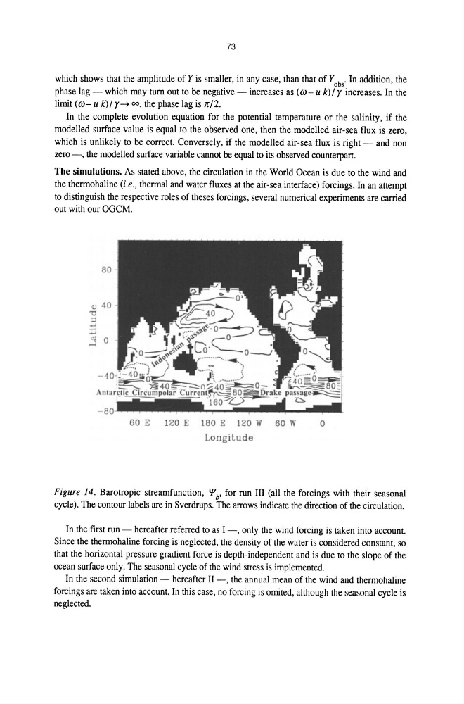
Figure 14. Barotropic streamfunction, 'l'h' for run III (all the forcings with their seasonal
cycle). The contour labels are in Sverdrups. The arrows indicate the direction of the circulation.
In the first run - hereafter referred to as I -, only the wind forcing is taken into account.
Since the thennohaline forcing is neglected, the density of the water is considered constant, so
that the horizontal pressure gradient force is depth-independent and is due to the slope of the
ocean surface only. The seasonal cycle of the wind stress is implemented.
In the second simulation - hereafter II -, the annual mean of the wind and thennohaline
forcings are taken into account. In this case, no forcing is omited, although the seasonal cycle is
neglected.
which shows that the amplitude of f is smaller, in any case, than that of fobs. In addition, the
phase lag - which may turn out to be negative - increases as (w - u k) I y increases. In the
limit (w- u k)/Y~ 00, the phase lag is n/2.
In the complete evolution equation for the potential temperature or the salinity, if the
modelled surface value is equal to the observed one, then the modelled air-sea flux is zero,
which is unlikely to be correct. Conversely, if the modelled air-sea flux is right - and non
zero -, the modelled surface variable cannot be equal to its observed counterpart.
The simulations. As stated above, the circulation in the World Ocean is due to the wind and
the thennohaline (i.e., thennal and water fluxes at the air-sea interface) forcings. In an attempt
to distinguish the respective roles of theses forcings, several numerical experiments are carried
out with our OGCM.
60E
120E 180E 120W
60W
0
Longitude
Figure 14. Barotropic streamfunction, 'l'h' for run III (all the forcings with their seasonal
cycle). The contour labels are in Sverdrups. The arrows indicate the direction of the circulation.
In the first run - hereafter referred to as I -, only the wind forcing is taken into account.
Since the thennohaline forcing is neglected, the density of the water is considered constant, so
that the horizontal pressure gradient force is depth-independent and is due to the slope of the
ocean surface only. The seasonal cycle of the wind stress is implemented.
In the second simulation - hereafter II -, the annual mean of the wind and thennohaline
forcings are taken into account. In this case, no forcing is omited, although the seasonal cycle is
neglected.