

71
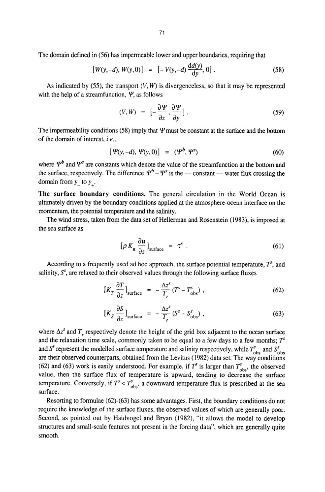
The domain defined in (56) has impenneable lower and upper boundaries, requiring that
[W(Y,-d), W(y,O)] = [- V(y,-d) d~?), 01.
(58)
As indicated by (55), the transport (V, W) is divergenceless, so that it may be represented
with the help of a streamfunction, lJ', as follows
(59)
The impenneability conditions (58) imply that 'f'must be constant at the surface and the bottom
of the domain of interest, i.e.,
['f'(y,-d), 'f'(y,0)] = ('f'h, 'f'S)
(60)
where ph and 'f's are constants which denote the value of the streamfunction at the bottom and
the surface, respectively. The difference 'f'h - 'f's is the - constant - water flux crossing the
domain from y _ to y +'
The surface boundary conditions. The general circulation in the World Ocean is
ultimately driven by the boundary conditions applied at the atmosphere-ocean interface on the
momentum, the potential temperature and the salinity.
The wind stress, taken from the data set of Hellerman and Rosenstein (1983), is imposed at
the sea surface as
[
au]
S
K -
= 1:
P u aZ surface
.
(61)
According to a frequently used ad hoc approach, the surface potential temperature, 1", and
salinity, SS, are relaxed to their observed values through the following surface fluxes
(62)
[K as]
_ _ dz s (SS _ ss )
S az surface - Tr
obs '
(63)
where dz s and Tr respectively denote the height of the grid box adjacent to the ocean surface
and the relaxation time scale, commonly taken to be equal to a few days to a few months; 1"
and SS represent the modelled surface temperature and salinity respectively, while 1"b and SSb
o s
0 s
are their observed counterparts, obtained from the Levitus (1982) data set. The way conditions
(62) and (63) work is easily understood. For example, if 1" is larger than T~bs' the observed
value, then the surface flux of temperature is upward, tending to decrease the surface
temperature. Conversely, if 1" < ~bs' a downward temperature flux is prescribed at the sea
surface.
Resorting to formulae (62)-(63) has some advantages. First, the boundary conditions do not
require the knowledge of the surface fluxes, the observed values of which are generally poor.
Second, as pointed out by Haidvogel and Bryan (1982), "it allows the model to develop
structures and small-scale features not present in the forcing data", which are generally quite
smooth.
The domain defined in (56) has impenneable lower and upper boundaries, requiring that
[W(Y,-d), W(y,O)] = [- V(y,-d) d~?), 01.
(58)
As indicated by (55), the transport (V, W) is divergenceless, so that it may be represented
with the help of a streamfunction, lJ', as follows
(59)
The impenneability conditions (58) imply that 'f'must be constant at the surface and the bottom
of the domain of interest, i.e.,
['f'(y,-d), 'f'(y,0)] = ('f'h, 'f'S)
(60)
where ph and 'f's are constants which denote the value of the streamfunction at the bottom and
the surface, respectively. The difference 'f'h - 'f's is the - constant - water flux crossing the
domain from y _ to y +'
The surface boundary conditions. The general circulation in the World Ocean is
ultimately driven by the boundary conditions applied at the atmosphere-ocean interface on the
momentum, the potential temperature and the salinity.
The wind stress, taken from the data set of Hellerman and Rosenstein (1983), is imposed at
the sea surface as
[
au]
S
K -
= 1:
P u aZ surface
.
(61)
According to a frequently used ad hoc approach, the surface potential temperature, 1", and
salinity, SS, are relaxed to their observed values through the following surface fluxes
(62)
[K as]
_ _ dz s (SS _ ss )
S az surface - Tr
obs '
(63)
where dz s and Tr respectively denote the height of the grid box adjacent to the ocean surface
and the relaxation time scale, commonly taken to be equal to a few days to a few months; 1"
and SS represent the modelled surface temperature and salinity respectively, while 1"b and SSb
o s
0 s
are their observed counterparts, obtained from the Levitus (1982) data set. The way conditions
(62) and (63) work is easily understood. For example, if 1" is larger than T~bs' the observed
value, then the surface flux of temperature is upward, tending to decrease the surface
temperature. Conversely, if 1" < ~bs' a downward temperature flux is prescribed at the sea
surface.
Resorting to formulae (62)-(63) has some advantages. First, the boundary conditions do not
require the knowledge of the surface fluxes, the observed values of which are generally poor.
Second, as pointed out by Haidvogel and Bryan (1982), "it allows the model to develop
structures and small-scale features not present in the forcing data", which are generally quite
smooth.