

397
BtT +"V. (TU)
FT(T) - "?(T - To).
(2)
B,S + "V. (SU)
FS(S) - -'1"'(5 - So),
(3)
BzP
-pg,
(4)
"V·U
0,
(5)
p
p(T,S,P),
(6)
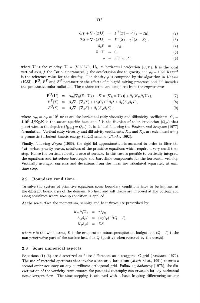
where U is the velocity, U = (U, V, W), Uh its horizontal projection (U, V), k is the local
vertical axis, f the Coriolis parameter, 9 the acceleration due to gravity and PO = 1020 Kg/m 3
is the reference value for the density. The density p is computed by the algorithm in Unesco
(1983). F U , FT and F S parametrize the effects of sub-grid mixing processes and FT includes
the penetrative solar radiation. These three terms are computed from the expressions:
Am["V h("V . U h) - "V x ("V h x Uh)] + Bz(KmBzUh),
Ap"V' ("VhT) + (poCp)-lBz1 + 8z(Kp8zT),
Ap"V' ("VhS) + 8z(K p8zS),
(7)
(8)
(9)
where Am = Ap = 10 3 m 2 Is are the horizontal eddy viscosity and diffusivity coefficients, Cp =
4.10 3 J IKg.K is the ocean specific heat and I is the fraction of solar irradiation (Q sr) that
penetrates to the depth z (l[z=oJ = Q sr). It is defined following the Pa,ulson a,nd Simpson (1977)
formulation. Vertical eddy viscosity and diffusivity coefficients, Km and K p , are calculated using
a pronostic turbulent kinetic energy (TKE) scheme (Bla,nke, 1992).
Finally, following Brya,n (1969), the rigid lid approximation is assumed in order to filter the
fast surface gravity waves, solutions of the primitive equations which require a very small time
step_ Hence the vertical velocity is zero at surface. In this case is possible to vertically integrate
the equations and introduce barotropic and baroclinic components for the horizontal velocity.
Vertically averaged currents and deviations from the mean are calculated separately at each
time step.
2.2 Boundary conditions.
To solve the system of primitive equations some boundary conditions have to be imposed at
the different boundaries of the domain. No heat and salt fluxes are imposed at the bottom and
along coastlines where no-slip condition is applied.
At the sea surface the momentum, salinity and heat fluxes are prescribed by:
Km. 8z U h
K p8 z T
K p 8 z S
T / po,
(POCp)-l(Q - 1),
ES,
where T is the wind stress, E is the evaporation minus precipitation budget and (Q - 1) is the
non-penetrative part of the surface heat flux Q (positive when received by the ocean).
2.3 Some numerical aspects.
Equations (1)-(6) are discretized as finite differences on a staggered C grid (Amkawa" 1972).
The use of vectorial operators that involve a tensorial formalism (Ma,rli et aL, 1991) ensures a
second order accuracy on any curvilinear orthogonal grid. Following Sa,doumy (1975), the discretization of the vorticity term ensures the potential enstrophy conservation for any horizontal
non-divergent flow. The time stepping is achieved with a basic leapfrog differencing scheme
BtT +"V. (TU)
FT(T) - "?(T - To).
(2)
B,S + "V. (SU)
FS(S) - -'1"'(5 - So),
(3)
BzP
-pg,
(4)
"V·U
0,
(5)
p
p(T,S,P),
(6)
where U is the velocity, U = (U, V, W), Uh its horizontal projection (U, V), k is the local
vertical axis, f the Coriolis parameter, 9 the acceleration due to gravity and PO = 1020 Kg/m 3
is the reference value for the density. The density p is computed by the algorithm in Unesco
(1983). F U , FT and F S parametrize the effects of sub-grid mixing processes and FT includes
the penetrative solar radiation. These three terms are computed from the expressions:
Am["V h("V . U h) - "V x ("V h x Uh)] + Bz(KmBzUh),
Ap"V' ("VhT) + (poCp)-lBz1 + 8z(Kp8zT),
Ap"V' ("VhS) + 8z(K p8zS),
(7)
(8)
(9)
where Am = Ap = 10 3 m 2 Is are the horizontal eddy viscosity and diffusivity coefficients, Cp =
4.10 3 J IKg.K is the ocean specific heat and I is the fraction of solar irradiation (Q sr) that
penetrates to the depth z (l[z=oJ = Q sr). It is defined following the Pa,ulson a,nd Simpson (1977)
formulation. Vertical eddy viscosity and diffusivity coefficients, Km and K p , are calculated using
a pronostic turbulent kinetic energy (TKE) scheme (Bla,nke, 1992).
Finally, following Brya,n (1969), the rigid lid approximation is assumed in order to filter the
fast surface gravity waves, solutions of the primitive equations which require a very small time
step_ Hence the vertical velocity is zero at surface. In this case is possible to vertically integrate
the equations and introduce barotropic and baroclinic components for the horizontal velocity.
Vertically averaged currents and deviations from the mean are calculated separately at each
time step.
2.2 Boundary conditions.
To solve the system of primitive equations some boundary conditions have to be imposed at
the different boundaries of the domain. No heat and salt fluxes are imposed at the bottom and
along coastlines where no-slip condition is applied.
At the sea surface the momentum, salinity and heat fluxes are prescribed by:
Km. 8z U h
K p8 z T
K p 8 z S
T / po,
(POCp)-l(Q - 1),
ES,
where T is the wind stress, E is the evaporation minus precipitation budget and (Q - 1) is the
non-penetrative part of the surface heat flux Q (positive when received by the ocean).
2.3 Some numerical aspects.
Equations (1)-(6) are discretized as finite differences on a staggered C grid (Amkawa" 1972).
The use of vectorial operators that involve a tensorial formalism (Ma,rli et aL, 1991) ensures a
second order accuracy on any curvilinear orthogonal grid. Following Sa,doumy (1975), the discretization of the vorticity term ensures the potential enstrophy conservation for any horizontal
non-divergent flow. The time stepping is achieved with a basic leapfrog differencing scheme