

344
1.4. A simplified ice-water model
In general, a glacier may have melt regions and a model taking into account the mechanical effects is very complicated, since we need to include an additional free boundary,
the ice-water interface which is "a priori" unknown.
This corresponds to the classical Stefan problem, that can be obtained from the energy
equation (1.10) under the assumption of the shallow-ice approximation with unidirectional
constant velocity. In dimensionless variables we have from (1.10), with v = 0 and neglecting the heat sources:
EM] + 8s'f) = l:!.'B in w x R ,
(1.24)
where v = B(x, z, s, t) with (x, z) Ewe R2 and (s, t) E R = ]0, S[ x ]0, T[, denotes the
temperature. We supose that B is normalized so that B = 0 is the melting temperature,
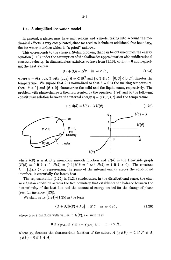
then {B < O} and {B > O} characterize the solid and the liquid zones, respectively. The
problem with phase change is then represented by the equation (1.24) and by the following
constitutive relation between the internal energy 'f) = 'f)(x, z, s, t) and the temperature
'f) E f3(B) = b(B) +,\ H(B) ,
(1.25)
b(B)+'\
H(B)
1-----B
b(B)
where b(B) is a strictly monotone smooth function and H(B) is the Heaviside graph
(H(B) = 0 if B < 0, H(B) = [0,11 if B = 0 and H(B) = 1 if B > 0). The constant
,\ = ['f)]o=o > 0, representing the jump of the internal energy across the solid-liquid
interface, is essentially the latent heat.
The representation (1.25) in (1.24) condensates, in the distributional sense, the classical Stefan condition accross the free boundary that establishes the balance between the
discontinuity of the heat flux and the amount of energy needed for the change of phase
(see, for instance, [R3]).
We shall write (1.24)-(1.25) in the form
(8t +8s )[b(B)+'\X]=l:!.'B III wxR,
where X is a function with values in H(B), i.e. such that
o ::; X{o>O} ::; X ::; 1 - X{9
XA(P) = 0 if P ~ A).
(1.26)
1 if PEA,
1.4. A simplified ice-water model
In general, a glacier may have melt regions and a model taking into account the mechanical effects is very complicated, since we need to include an additional free boundary,
the ice-water interface which is "a priori" unknown.
This corresponds to the classical Stefan problem, that can be obtained from the energy
equation (1.10) under the assumption of the shallow-ice approximation with unidirectional
constant velocity. In dimensionless variables we have from (1.10), with v = 0 and neglecting the heat sources:
EM] + 8s'f) = l:!.'B in w x R ,
(1.24)
where v = B(x, z, s, t) with (x, z) Ewe R2 and (s, t) E R = ]0, S[ x ]0, T[, denotes the
temperature. We supose that B is normalized so that B = 0 is the melting temperature,
then {B < O} and {B > O} characterize the solid and the liquid zones, respectively. The
problem with phase change is then represented by the equation (1.24) and by the following
constitutive relation between the internal energy 'f) = 'f)(x, z, s, t) and the temperature
'f) E f3(B) = b(B) +,\ H(B) ,
(1.25)
b(B)+'\
H(B)
1-----B
b(B)
where b(B) is a strictly monotone smooth function and H(B) is the Heaviside graph
(H(B) = 0 if B < 0, H(B) = [0,11 if B = 0 and H(B) = 1 if B > 0). The constant
,\ = ['f)]o=o > 0, representing the jump of the internal energy across the solid-liquid
interface, is essentially the latent heat.
The representation (1.25) in (1.24) condensates, in the distributional sense, the classical Stefan condition accross the free boundary that establishes the balance between the
discontinuity of the heat flux and the amount of energy needed for the change of phase
(see, for instance, [R3]).
We shall write (1.24)-(1.25) in the form
(8t +8s )[b(B)+'\X]=l:!.'B III wxR,
where X is a function with values in H(B), i.e. such that
o ::; X{o>O} ::; X ::; 1 - X{9
XA(P) = 0 if P ~ A).
(1.26)
1 if PEA,