

324
3 Large scale fluctuations
3.1 Waves on glaciers
Waves on glaciers are mostly easily understood by considering an isothermal, two-dimensional
model. We suppose the base is flat (h = 0), so that equations (2.20) and (2.21) give
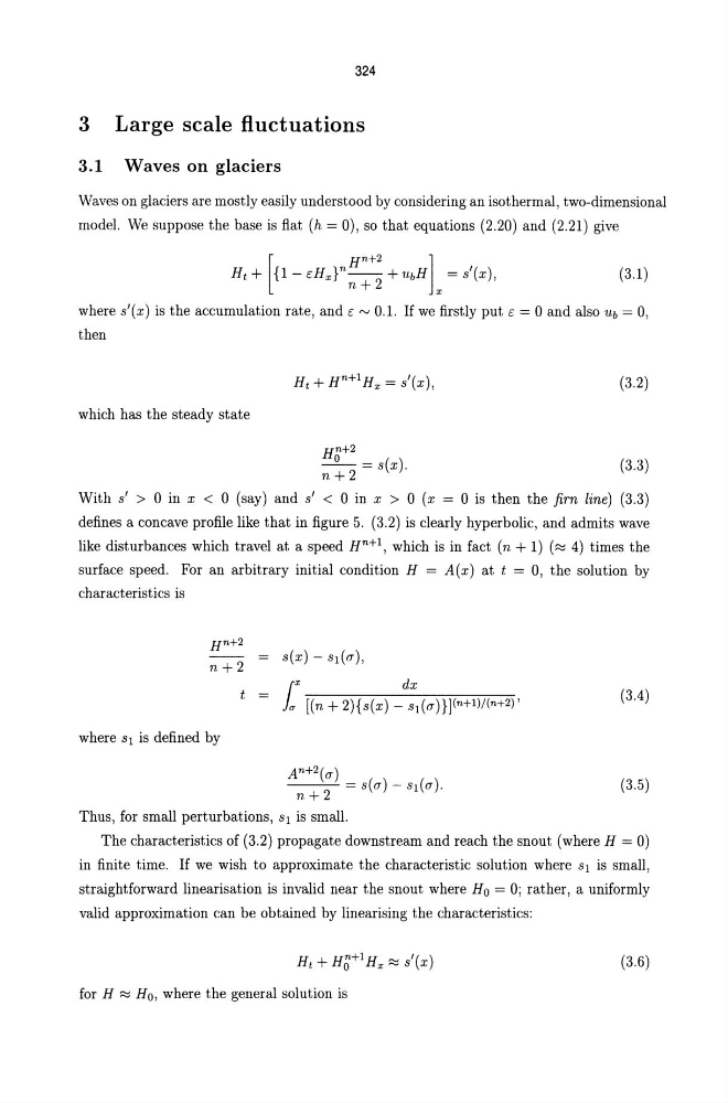
Ht + [{1 - EHx }"H
n +
2
+ U,bH] = s'(x),
n +2
x
(3.1)
where s'(x) is the accumulation rate, and E ~ 0.1. If we firstly put E = 0 and also U,b = 0,
then
which has the steady state
H n + 2
_0 _ = s(x).
n+2
(3.2)
(3.3)
With s' > 0 in x < 0 (say) and s' < 0 in x > 0 (x = 0 is then the jim line) (3.3)
defines a concave profile like that in figure 5. (3.2) is dearly hyperbolic, and admits wave
like disturbances which travel at a speed H n +1, which is in fact (n + 1) (~ 4) times the
surface speed. For an arbitrary initial condition H = A(x) at t = 0, the solution by
characteristics is
t
dx
}IT [(n + 2){s(x) - s1(a)}](n+1)/(n+2) ,
(3.4)
where S1 is defined by
(3.5)
Thus, for small perturbations, S1 is small.
The characteristics of (3.2) propagate downstream and reach the snout (where H = 0)
in finite time. If we wish to approximate the characteristic solution where S1 is small,
straightforward linearisation is invalid near the snout where H o = 0; rather, a uniformly
valid approximation can be obtained by linearising the characteristics:
(3.6)
for H ~ Ho, where the general solution is
3 Large scale fluctuations
3.1 Waves on glaciers
Waves on glaciers are mostly easily understood by considering an isothermal, two-dimensional
model. We suppose the base is flat (h = 0), so that equations (2.20) and (2.21) give
Ht + [{1 - EHx }"H
n +
2
+ U,bH] = s'(x),
n +2
x
(3.1)
where s'(x) is the accumulation rate, and E ~ 0.1. If we firstly put E = 0 and also U,b = 0,
then
which has the steady state
H n + 2
_0 _ = s(x).
n+2
(3.2)
(3.3)
With s' > 0 in x < 0 (say) and s' < 0 in x > 0 (x = 0 is then the jim line) (3.3)
defines a concave profile like that in figure 5. (3.2) is dearly hyperbolic, and admits wave
like disturbances which travel at a speed H n +1, which is in fact (n + 1) (~ 4) times the
surface speed. For an arbitrary initial condition H = A(x) at t = 0, the solution by
characteristics is
t
dx
}IT [(n + 2){s(x) - s1(a)}](n+1)/(n+2) ,
(3.4)
where S1 is defined by
(3.5)
Thus, for small perturbations, S1 is small.
The characteristics of (3.2) propagate downstream and reach the snout (where H = 0)
in finite time. If we wish to approximate the characteristic solution where S1 is small,
straightforward linearisation is invalid near the snout where H o = 0; rather, a uniformly
valid approximation can be obtained by linearising the characteristics:
(3.6)
for H ~ Ho, where the general solution is