

155
(II.l,l)
Q is an open subset of R 2, connected, of boundary ' Y of class C 1,1 ory is a
convex polygon; ' Y has a finite number of connected components ' Y i , i = O ... n, ' YO indicating
the boundary of the infinite connected component of the complementary of Q in R2. The
equations of the studied model are the following.
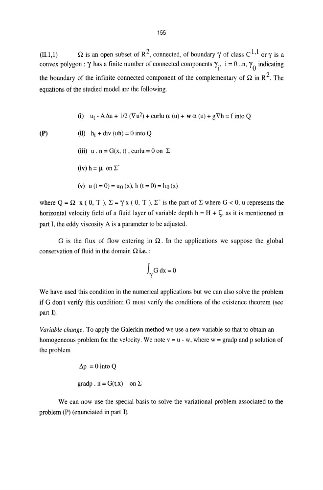
(i) Ut - A~u + 112 (Vu 2 ) + curlu a (u) + wa (u) + gVh == f into Q
(P)
(ii) ht + div (uh) = 0 into Q
(iii) u. n = G(x, t) , curlu = 0 on L
(iv) h = I.l on L(v) u (t = 0) == uo (x), h (t = 0) == ho (x)
where Q = Q x ( 0, T ), L == ' Y x ( 0, T ), L- is the part of L where G < 0, u represents the
horizontal velocity field of a fluid layer of variable depth h = H + ~, as it is mentionned in
part I, the eddy viscosity A is a parameter to be adjusted.
G is the flux of flow entering in Q. In the applications we suppose the global
conservation of fluid in the domain Q i.e. :
f Gdx==O
' Y
We have used this condition in the numerical applications but we can also solve the problem
if G don't verify this condition; G must verify the conditions of the existence theorem (see
part I).
Variable change. To apply the Galerkin method we use a new variable so that to obtain an
homogeneous problem for the velocity. We note v == u - w, where w == gradp and p solution of
the problem
~p =Ointo Q
gradp . n = G(t,x) on L
We can now use the special basis to solve the variational problem associated to the
problem (P) (enunciated in part I).
(II.l,l)
Q is an open subset of R 2, connected, of boundary ' Y of class C 1,1 ory is a
convex polygon; ' Y has a finite number of connected components ' Y i , i = O ... n, ' YO indicating
the boundary of the infinite connected component of the complementary of Q in R2. The
equations of the studied model are the following.
(i) Ut - A~u + 112 (Vu 2 ) + curlu a (u) + wa (u) + gVh == f into Q
(P)
(ii) ht + div (uh) = 0 into Q
(iii) u. n = G(x, t) , curlu = 0 on L
(iv) h = I.l on L(v) u (t = 0) == uo (x), h (t = 0) == ho (x)
where Q = Q x ( 0, T ), L == ' Y x ( 0, T ), L- is the part of L where G < 0, u represents the
horizontal velocity field of a fluid layer of variable depth h = H + ~, as it is mentionned in
part I, the eddy viscosity A is a parameter to be adjusted.
G is the flux of flow entering in Q. In the applications we suppose the global
conservation of fluid in the domain Q i.e. :
f Gdx==O
' Y
We have used this condition in the numerical applications but we can also solve the problem
if G don't verify this condition; G must verify the conditions of the existence theorem (see
part I).
Variable change. To apply the Galerkin method we use a new variable so that to obtain an
homogeneous problem for the velocity. We note v == u - w, where w == gradp and p solution of
the problem
~p =Ointo Q
gradp . n = G(t,x) on L
We can now use the special basis to solve the variational problem associated to the
problem (P) (enunciated in part I).