

362
8 Waves
φ = 60
◦
=
π
3
rad
x =
φ
k
=
π/3
4π/3
= 0.25 m
(b) φ = ωt = (500π)(10 −3 ) =
π
2
rad = 90 ◦
8.13 y 1 = A 1 sin(kx − ωt)
y 2 = A 2 sin
kx − ωt +
π
2
= A 2 cos(kx − ωt)
y = y 1 + y 2
= A 1 sin(kx − ωt) + A 2 cos(kx − ωt)
=
A 2
1 + A 2
2
⎡
⎣
A 1
A 2
1 + A 2
2
sin(kx − ωt) +
A 2
A 2
1 + A 2
2
cos(kx − ωt)
⎤
⎦
Put
A 1
A 2
1 + A 2
2
= cos α. Then
A 2
A 2
1 + A 2
2
= sin α
∴ y =
A 2
1 + A 2
2 [sin(kx − ωt) cos α + cos(kx − ωt) sin α]
=
A 2
1 + A 2
2 sin(kx − ωt + α)
which has the amplitude A =
A 2
1 + A 2
2 =
√
6 2 + 8 2 = 10 cm.
Graphical Method
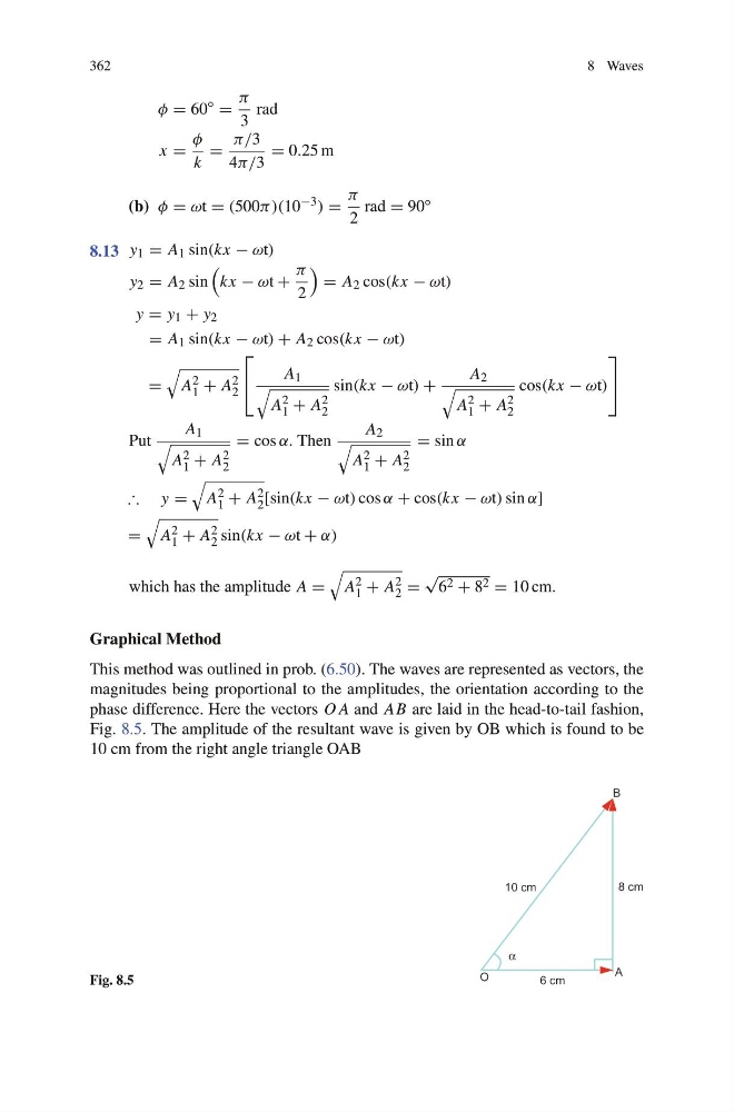
This method was outlined in prob. (6.50). The waves are represented as vectors, the
magnitudes being proportional to the amplitudes, the orientation according to the
phase difference. Here the vectors O A and AB are laid in the head-to-tail fashion,
Fig. 8.5. The amplitude of the resultant wave is given by OB which is found to be
10 cm from the right angle triangle OAB
Fig. 8.5
8 Waves
φ = 60
◦
=
π
3
rad
x =
φ
k
=
π/3
4π/3
= 0.25 m
(b) φ = ωt = (500π)(10 −3 ) =
π
2
rad = 90 ◦
8.13 y 1 = A 1 sin(kx − ωt)
y 2 = A 2 sin
kx − ωt +
π
2
= A 2 cos(kx − ωt)
y = y 1 + y 2
= A 1 sin(kx − ωt) + A 2 cos(kx − ωt)
=
A 2
1 + A 2
2
⎡
⎣
A 1
A 2
1 + A 2
2
sin(kx − ωt) +
A 2
A 2
1 + A 2
2
cos(kx − ωt)
⎤
⎦
Put
A 1
A 2
1 + A 2
2
= cos α. Then
A 2
A 2
1 + A 2
2
= sin α
∴ y =
A 2
1 + A 2
2 [sin(kx − ωt) cos α + cos(kx − ωt) sin α]
=
A 2
1 + A 2
2 sin(kx − ωt + α)
which has the amplitude A =
A 2
1 + A 2
2 =
√
6 2 + 8 2 = 10 cm.
Graphical Method
This method was outlined in prob. (6.50). The waves are represented as vectors, the
magnitudes being proportional to the amplitudes, the orientation according to the
phase difference. Here the vectors O A and AB are laid in the head-to-tail fashion,
Fig. 8.5. The amplitude of the resultant wave is given by OB which is found to be
10 cm from the right angle triangle OAB
Fig. 8.5