

RC Circuits
In preceding modules we dealt only with circuits in which the currents did not
vary with time. Here we begin a discussion of time-varying currents.
Charging a Capacitor
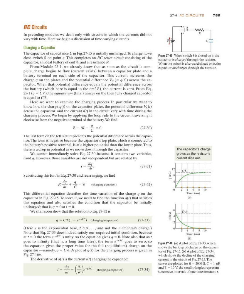
The capacitor of capacitance C in Fig. 27-15 is initially uncharged. To charge it, we
close switch S on point a. This completes an RC series circuit consisting of the
capacitor, an ideal battery of emf Ᏹ, and a resistance R.
From Module 25-1, we already know that as soon as the circuit is complete, charge begins to flow (current exists) between a capacitor plate and a
battery terminal on each side of the capacitor. This current increases the
charge q on the plates and the potential difference V C (ϭ q/C) across the capacitor. When that potential difference equals the potential difference across
the battery (which here is equal to the emf Ᏹ), the current is zero. From Eq.
25-1 (q ϭ CV), the equilibrium (final) charge on the then fully charged capacitor
is equal to C Ᏹ.
Here we want to examine the charging process. In particular we want to
know how the charge q(t) on the capacitor plates, the potential difference V C (t)
across the capacitor, and the current i(t) in the circuit vary with time during the
charging process. We begin by applying the loop rule to the circuit, traversing it
clockwise from the negative terminal of the battery. We find
(27-30)
The last term on the left side represents the potential difference across the capacitor. The term is negative because the capacitor’s top plate, which is connected to
the battery’s positive terminal, is at a higher potential than the lower plate. Thus,
there is a drop in potential as we move down through the capacitor.
We cannot immediately solve Eq. 27-30 because it contains two variables,
i and q. However, those variables are not independent but are related by
(27-31)
Substituting this for i in Eq. 27-30 and rearranging, we find
(charging equation).
(27-32)
This differential equation describes the time variation of the charge q on the
capacitor in Fig. 27-15. To solve it, we need to find the function q(t) that satisfies
this equation and also satisfies the condition that the capacitor be initially
uncharged; that is, q ϭ 0 at t ϭ 0.
We shall soon show that the solution to Eq. 27-32 is
q ϭ C Ᏹ(1 Ϫ e
Ϫt/RC
) (charging a capacitor).
(27-33)
(Here e is the exponential base, 2.718 . . . , and not the elementary charge.)
Note that Eq. 27-33 does indeed satisfy our required initial condition, because
at t ϭ 0 the term e
Ϫt/RC
is unity; so the equation gives q ϭ 0. Note also that as t
goes to infinity (that is, a long time later), the term e
Ϫt/RC
goes to zero; so
the equation gives the proper value for the full (equilibrium) charge on the
capacitor — namely, q ϭ C Ᏹ. A plot of q(t) for the charging process is given in
Fig. 27-16a.
The derivative of q(t) is the current i(t) charging the capacitor:
(charging a capacitor).
(27-34)
i ϭ
dq
dt
ϭ
Ᏹ
R e
Ϫt/RC
R
dq
dt
ϩ
q
C
ϭ Ᏹ
i ϭ
dq
dt
.
Ᏹ Ϫ iR Ϫ
q
C
ϭ 0.
789
27-4 RC CI RCU ITS
Figure 27-15 When switch S is closed on a, the
capacitor is charged through the resistor.
When the switch is afterward closed on b, the
capacitor discharges through the resistor.
C
+
–
S
R
b
a
Figure 27-16 (a) A plot of Eq. 27-33, which
shows the buildup of charge on the capacitor of Fig. 27-15. (b) A plot of Eq. 27-34,
which shows the decline of the charging
current in the circuit of Fig. 27-15. The
curves are plotted for R ϭ 2000 ⍀, C ϭ 1 mF,
and Ᏹ ϭ 10 V; the small triangles represent
successive intervals of one time constant t.
q ( C)
12
i (mA)
6
8
4
4
2
0
0
2 4 6 8 10
2 4 6 8
Time (ms)
Time (ms)
(a)
(b)
10
µ
C
/R
The capacitor’s charge
grows as the resistor’s
current dies out.