

674
CHAPTE R 23 GAUSS’ L AW
Sample Problem 23.07 Electric field near two parallel nonconducting sheets with charge
Figure 23-19a shows portions of two large, parallel, nonconducting sheets, each with a fixed uniform charge on one
side. The magnitudes of the surface charge densities are
s (ϩ) ϭ 6.8 mC/m
2
for the positively charged sheet and s (Ϫ) ϭ
4.3 mC/m
2
for the negatively charged sheet.
Find the electric field
(a) to the left of the sheets,
(b) between the sheets, and (c) to the right of the sheets.
KEY IDEA
With the charges fixed in place (they are on nonconductors),
we can find the electric field of the sheets in Fig. 23-19a by
(1) finding the field of each sheet as if that sheet were isolated
and (2) algebraically adding the fields of the isolated sheets
E
:
(a)
–
–
–
–
–
–
–
–
–
–
+
+
+
+
+
+
+
+
+
+
+
+
+
+
+
σ (+)
σ (–)
(b)
B
E(–)
R
E(–)
L
E(+)
–
–
–
–
–
–
–
–
–
–
+
+
+
+
+
+
+
+
+
+
+
+
+
+
+
E(+)
E(+)
E(–)
(c)
E L
E B
E R
–
–
–
–
–
–
–
–
–
–
+
+
+
+
+
+
+
+
+
+
+
+
+
+
+
Figure 23-19 (a) Two large, parallel sheets, uniformly charged on
one side. (b) The individual
electric fields resulting from the
two charged sheets. (c) The net
field due to both charged
sheets, found by superposition.
+
+
+
+
+
σ 1
σ 1
+
+
+
+
+
–
σ 1
σ 1
–
–
–
–
–
–
–
–
–
σ
2 1
+
+
+
+
+
+
+
+
+
+
(c)
–
–
–
–
–
–
–
–
–
–
E = 0
E = 0
(a)
(b)
E
E
E
E
E
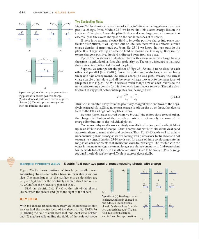
Figure 23-18 (a) A thin, very large conducting plate with excess positive charge.
(b) An identical plate with excess negative
charge. (c) The two plates arranged so
they are parallel and close.
Two Conducting Plates
Figure 23-18a shows a cross section of a thin, infinite conducting plate with excess
positive charge. From Module 23-3 we know that this excess charge lies on the
surface of the plate. Since the plate is thin and very large, we can assume that
essentially all the excess charge is on the two large faces of the plate.
If there is no external electric field to force the positive charge into some particular distribution, it will spread out on the two faces with a uniform surface
charge density of magnitude s 1 . From Eq. 23-11 we know that just outside the
plate this charge sets up an electric field of magnitude E ϭ s 1 /´ 0 . Because the
excess charge is positive, the field is directed away from the plate.
Figure 23-18b shows an identical plate with excess negative charge having
the same magnitude of surface charge density s 1 . The only difference is that now
the electric field is directed toward the plate.
Suppose we arrange for the plates of Figs. 23-18a and b to be close to each
other and parallel (Fig. 23-18c). Since the plates are conductors, when we bring
them into this arrangement, the excess charge on one plate attracts the excess
charge on the other plate, and all the excess charge moves onto the inner faces of
the plates as in Fig. 23-18c. With twice as much charge now on each inner face, the
new surface charge density (call it s) on each inner face is twice s 1 .Thus, the electric field at any point between the plates has the magnitude
(23-14)
This field is directed away from the positively charged plate and toward the negatively charged plate. Since no excess charge is left on the outer faces, the electric
field to the left and right of the plates is zero.
Because the charges moved when we brought the plates close to each other,
the charge distribution of the two-plate system is not merely the sum of the
charge distributions of the individual plates.
One reason why we discuss seemingly unrealistic situations, such as the field set
up by an infinite sheet of charge, is that analyses for “infinite” situations yield good
approximations to many real-world problems. Thus, Eq. 23-13 holds well for a finite
nonconducting sheet as long as we are dealing with points close to the sheet and not
too near its edges. Equation 23-14 holds well for a pair of finite conducting plates as
long as we consider points that are not too close to their edges. The trouble with the
edges is that near an edge we can no longer use planar symmetry to find expressions
for the fields. In fact, the field lines there are curved (said to be an edge effect or fringing), and the fields can be very difficult to express algebraically.
E ϭ
2s 1
´ 0
ϭ
s
´ 0
.