The Electric Field Due to an Electric Dipole
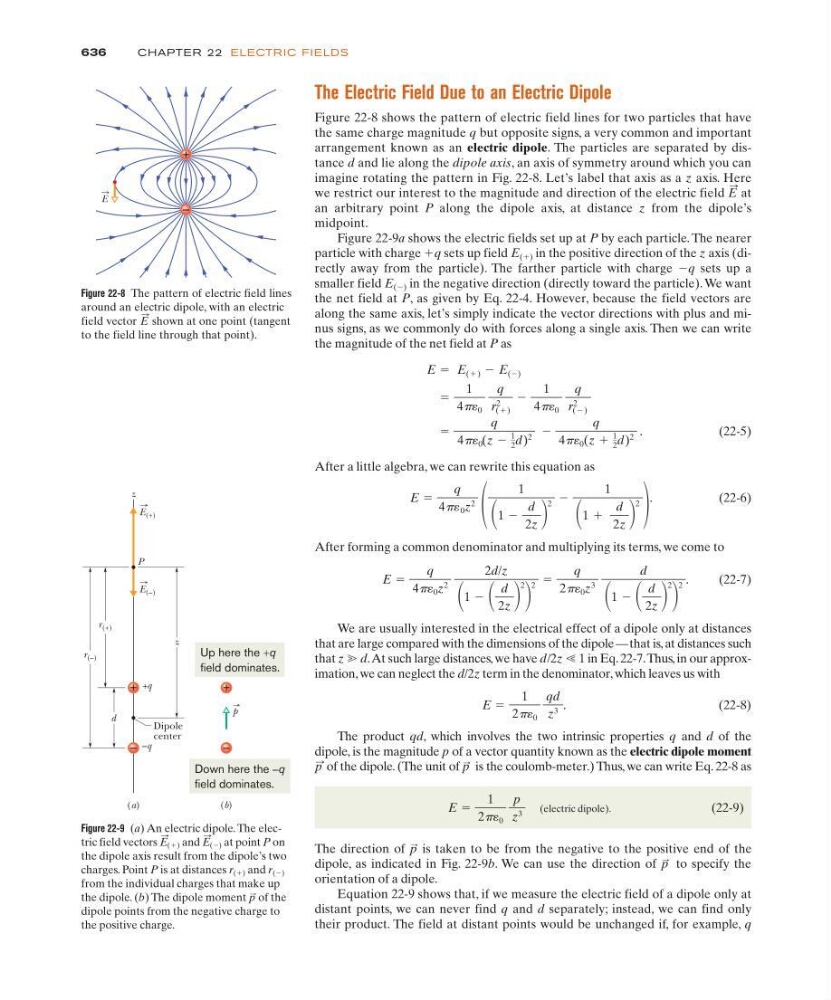
Figure 22-8 shows the pattern of electric field lines for two particles that have
the same charge magnitude q but opposite signs, a very common and important
arrangement known as an electric dipole. The particles are separated by distance d and lie along the dipole axis, an axis of symmetry around which you can
imagine rotating the pattern in Fig. 22-8. Let’s label that axis as a z axis. Here
we restrict our interest to the magnitude and direction of the electric field at
an arbitrary point P along the dipole axis, at distance z from the dipole’s
midpoint.
Figure 22-9a shows the electric fields set up at P by each particle. The nearer
particle with charge ϩq sets up field E (ϩ) in the positive direction of the z axis (directly away from the particle). The farther particle with charge Ϫq sets up a
smaller field E (Ϫ) in the negative direction (directly toward the particle). We want
the net field at P, as given by Eq. 22-4. However, because the field vectors are
along the same axis, let’s simply indicate the vector directions with plus and minus signs, as we commonly do with forces along a single axis. Then we can write
the magnitude of the net field at P as
(22-5)
After a little algebra, we can rewrite this equation as
(22-6)
After forming a common denominator and multiplying its terms, we come to
(22-7)
We are usually interested in the electrical effect of a dipole only at distances
that are large compared with the dimensions of the dipole — that is, at distances such
that z ӷ d.At such large distances, we have d/2z Ӷ 1 in Eq. 22-7.Thus, in our approximation, we can neglect the d/2z term in the denominator, which leaves us with
(22-8)
The product qd, which involves the two intrinsic properties q and d of the
dipole, is the magnitude p of a vector quantity known as the electric dipole moment
of the dipole. (The unit of is the coulomb-meter.) Thus, we can write Eq. 22-8 as
(electric dipole).
(22-9)
The direction of is taken to be from the negative to the positive end of the
dipole, as indicated in Fig. 22-9b. We can use the direction of
to specify the
orientation of a dipole.
Equation 22-9 shows that, if we measure the electric field of a dipole only at
distant points, we can never find q and d separately; instead, we can find only
their product. The field at distant points would be unchanged if, for example, q
p
:
p
:
E ϭ
1
2p´ 0
p
z
3
p
:
p
:
E ϭ
1
2p´ 0
qd
z
3
.
ϭ
q
2p´ 0 z
3
d
΂ 1 Ϫ ΂
d
2z ΃
2
΃
2
.
E ϭ
q
4p´ 0 z
2
2d/z
΂ 1 Ϫ ΂
d
2z ΃
2
΃
2
E ϭ
q
4p´ 0 z
2
΂
1
΂ 1 Ϫ
d
2z ΃
2
Ϫ
1
΂ 1 ϩ
d
2z ΃
2
΃
.
ϭ
q
4p´ 0 (z Ϫ
1
2 d)
2
Ϫ
q
4p´ 0 (z ϩ
1
2 d)
2
.
ϭ
1
4p´ 0
q
r
2
(ϩ)
Ϫ
1
4p´ 0
q
r
2
(Ϫ)
E ϭ E (ϩ) Ϫ E (Ϫ)
E
:
636
CHAPTE R 22 ELECTRIC FIELDS
Figure 22-9 (a) An electric dipole. The electric field vectors
and
at point P on
the dipole axis result from the dipole’s two
charges. Point P is at distances r (ϩ) and r (Ϫ)
from the individual charges that make up
the dipole. (b) The dipole moment of the
dipole points from the negative charge to
the positive charge.
p
:
E
:
(Ϫ)
E
:
(ϩ)
z
r (–)
r (+)
E (+)
d
z
–q
+q
P
(a)
(b)
+
+
–
–
p
E (–)
Dipole
center
Up here the +q
field dominates.
Down here the –q
field dominates.
Figure 22-8 The pattern of electric field lines
around an electric dipole, with an electric
field vector shown at one point (tangent
to the field line through that point).
E
:
+
–
E